Fisheries New Zealand standard grids

library(nzsf)
library(ggspatial)
library(stars)

theme_set(theme_bw() + theme(axis.title = element_blank()))

The process is:

Identify the area of interest (e.g., the New Zealand EEZ, a QMA)
Place a bounding box around the area of interest
Generate a standard grid, with the specified cell_size, that covers the bounding box

The standard grid can either be a simple feature collection of polygons (return_raster = FALSE) or a raster (return_raster = TRUE). The standard grid can extend beyond the range of the bounding box, depending on the cell_size.

Standard grids as polygons

eez <- get_statistical_areas(area = "EEZ", proj = proj_nzsf())
bb_eez <- st_bbox(eez) %>% st_as_sfc()
grd256_eez <- get_standard_grid(cell_size = 256, bounding_box = st_bbox(eez), 
                                return_raster = FALSE)
grd064_eez <- get_standard_grid(cell_size = 64, bounding_box = st_bbox(eez), 
                                return_raster = FALSE)

Plot and check with center point and bounding box

ggplot() +
  geom_sf(data = grd064_eez,  colour = "lightblue",  fill = NA, alpha = 0.15) +
  geom_sf(data = grd256_eez,  colour = "tomato",  fill = NA, alpha = 0.5) +
  plot_statistical_areas(area = "EEZ", colour = "black", fill = NA, linetype = "dashed") +
  geom_sf(data = bb_eez, colour = "red", fill = NA, linetype = "dashed") +
  plot_coast(resolution = "medium", fill = "black", colour = "black") +
  geom_point(aes(x = 0, y = -422600), colour = "green") + 
  plot_clip("NZ") +
  annotation_scale(location = "tr", unit_category = "metric")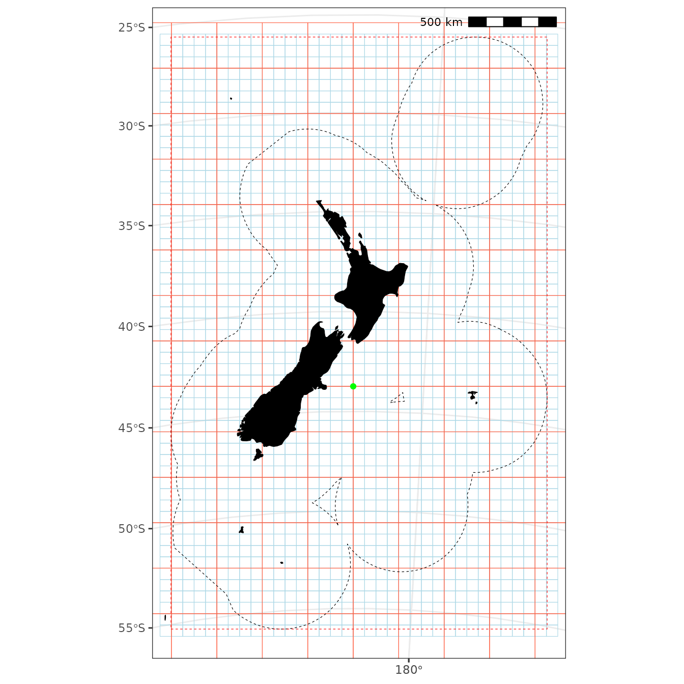

Figure 1: The New Zealand EEZ (dashed black lines), a box bounding the EEZ (dashed red lines), a 50 x 50 km grid (blue lines), a 200 x 200 km grid (red lines), and the origin (green point).

cra1 <- get_statistical_areas(area = "CRA", proj = proj_nzsf()) %>% 
  filter(QMA %in% "CRA1")

bb_cra1 <- st_bbox(cra1) %>% st_as_sfc()

grd256_cra1 <- get_standard_grid(cell_size = 256, bounding_box = st_bbox(cra1), 
                                 return_raster = FALSE)

grd064_cra1 <- get_standard_grid(cell_size = 64, bounding_box = st_bbox(cra1), 
                                 return_raster = FALSE)

ggplot() +
  geom_sf(data = grd064_cra1,  colour = "lightblue",  fill = NA, alpha = 0.5) +
  geom_sf(data = grd256_cra1,  colour = "tomato",  fill = NA, alpha = 0.5) +
  geom_sf(data = cra1, colour = "black", fill = NA, linetype = "dashed") +
  geom_sf(data = bb_cra1, colour = "red", fill = NA, linetype = "dashed") +
  plot_coast(resolution = "large", fill = "black", colour = "black") +
  annotation_scale(location = "tr", unit_category = "metric") +
  plot_clip(x = grd256_cra1)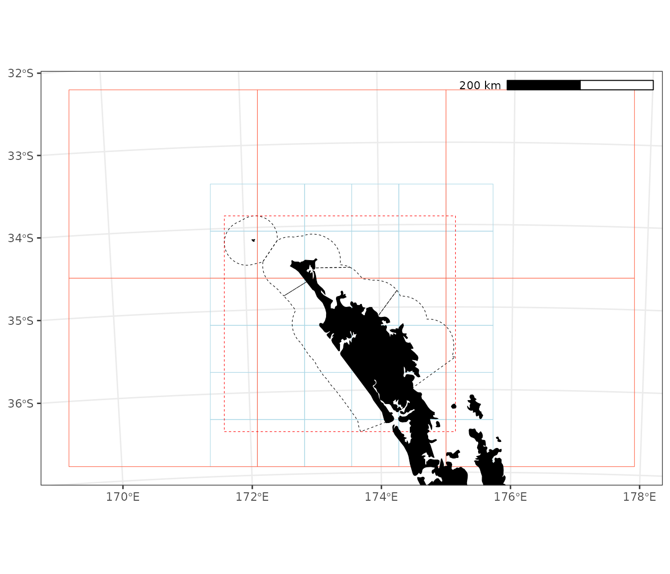

The CRA 1 QMA (dashed black), a box bounding around CRA 1 (dashed red), a 64 x 64 km grid (blue), and 256 x 256 km grid (red). Note that there is no point of origin shown as it is outside of the CRA 1 QMA.

Plot and check overlap of two grids.

ggplot() +
  geom_sf(data = grd256_eez,  colour = "lightblue",  fill = NA, alpha = 0.5) +
  geom_sf(data = cra1, colour = "orange", fill = NA) +
  geom_sf(data = grd256_cra1,  colour = "blue",  fill = NA, alpha = 0.5, linetype = "dashed") +
  geom_sf(data = grd064_cra1,  colour = "tomato",  fill = NA, alpha = 0.5, linetype = "dashed") +
  plot_coast(resolution = "high", fill = "black", colour = "black") +
  geom_point(aes(x = 0, y = -422600), colour = "green") +
  annotation_scale(location = "tr", unit_category = "metric") +
  coord_sf(xlim = c(-5e+05, 2.5e+05), ylim = c(-422600, 895400))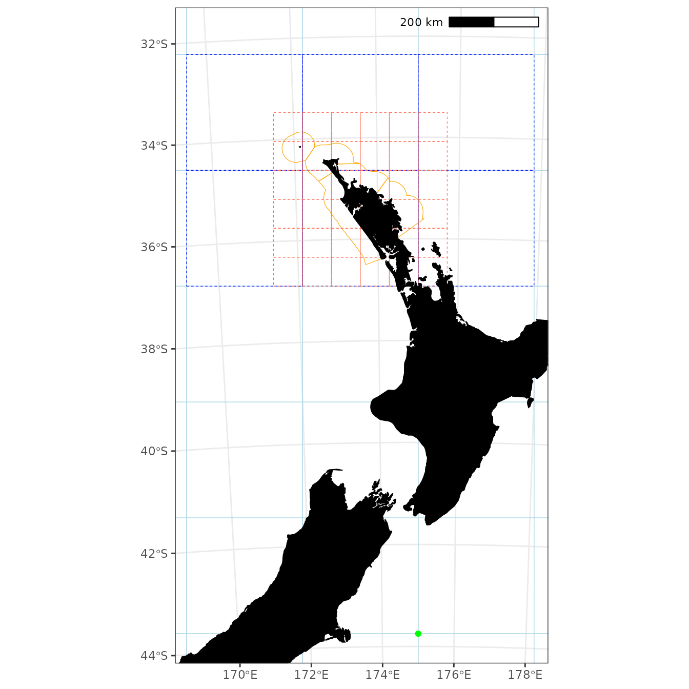

EEZ 200 x 200 km grid (light blue), CRA 1 200 x 200 km grid (dashed blue), origin (green point).

In the figure below, I show that you can specify the number of cells either side of the origin.

bb1 <- st_bbox(eez)
bb1[1] <- -150000 # xmin
bb1[2] <- -422600 - 3000 # ymin (3 cells below the origin)
bb1[3] <- 3000 # xmax (3 cells to the right of the origin)
bb1[4] <- -400000 # ymax

grd001_eez <- get_standard_grid(cell_size = 1, bounding_box = bb1, 
                                return_raster = FALSE)

# Plot and check center point at fine scale
ggplot() +
  geom_sf(data = grd001_eez,  colour = "lightblue",  fill = NA, alpha = 0.15) +
  plot_coast(resolution = "150k", fill = "black", colour = "black") +
  geom_point(aes(x = 0, y = -422600), colour = "green") + 
  annotation_scale(location = "tr", unit_category = "metric") +
  plot_clip(x = grd001_eez)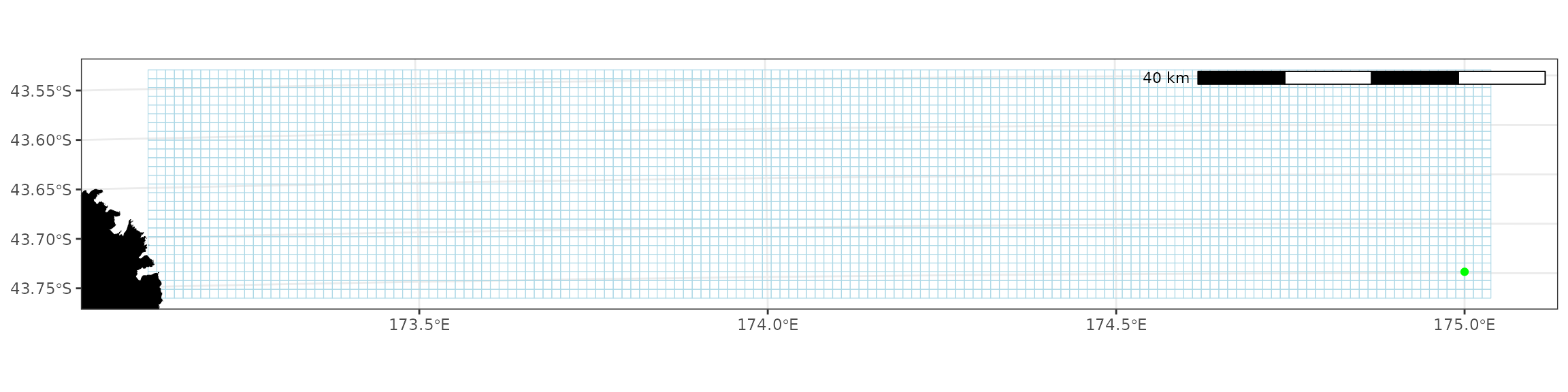

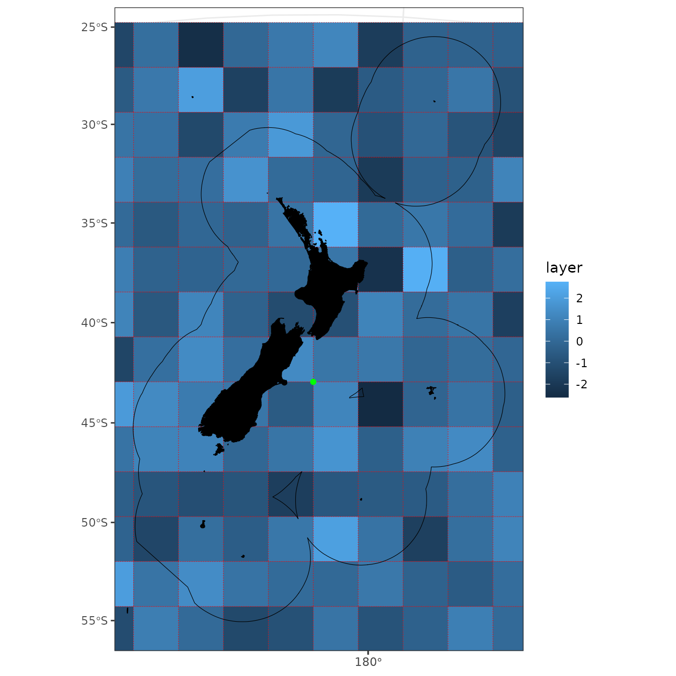
A 1 x 1 km grid (blue), origin (green point), and tip of Banks Peninsula to west. Note that the cell sizes agree well with the scale at top-right.

Standard grids as rasters

Rasters are more useful than polygons. Get standard grid as a raster. Fill the grid with random values and plot it.

r <- get_standard_grid(cell_size = 256, bounding_box = st_bbox(eez), 
                       return_raster = TRUE)
r[] <- rnorm(n = ncell(r))
rstar <- st_as_stars(r)

ggplot() +
  geom_stars(data = rstar) +
  geom_sf(data = grd256_eez, fill = NA, colour = "red", linetype = "dotted") +
  plot_coast(resolution = "large", fill = "black", colour = "black") +
  plot_statistical_areas(area = "EEZ", colour = "black", fill = NA) +
  geom_point(aes(x = 0, y = -422600), colour = "green") +
  plot_clip("NZ")

EEZ 200 x 200 km grid as polygons (dotted red), EEZ 200 x 200 km grid as raster (blue), origin (green point).

Darcy Webber, Sophie Mormede, Charles Edwards

Standard grids as polygons

Standard grids as rasters