---
title: "Data weighting"
format:
html:
toc: true
code-fold: true
code-tools: true
lightbox: true
favicon: ../images/favicon.svg
include-in-header:
text: |
<link rel="icon" href="../images/favicon.svg" type="image/svg+xml">
vignette: >
%\VignetteIndexEntry{Data weighting}
%\VignetteEncoding{UTF-8}
%\VignetteEngine{quarto::html}
bibliography: "references.bib"
link-citations: true
params:
force_refit: false
editor_options:
chunk_output_type: console
---
# Introduction
This document configures the current `sbt_model` RTMB model structure using the
ADMB selectivity functions from `sbt_vs_admb.qmd`. Fishery 7 shares the fishery
1 (LL1) selectivity. It is kept as a separate vignette so the default `sbt.qmd`
model setup and package code are unaffected.
::: {.callout-note}
## Scope of this comparison
This is a like-for-like diagnostic comparison built from the complete
package-default scientific example, not the selected ESC31 base assessment.
Its objectives, fitted parameters, and OSA summaries test selectivity and
data-weighting behavior within that example and must not be read as ESC31
acceptance diagnostics. The accepted assessment model and its residual
statistics are reported separately on the
[ESC31 base-model page](../ESC31/2_base.html).
:::
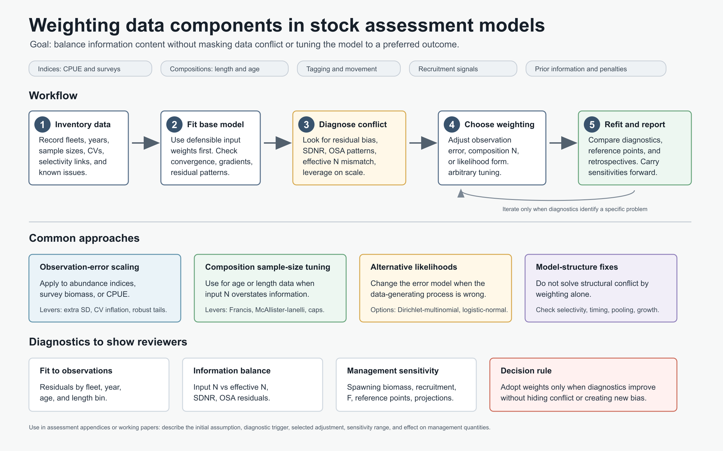{#fig-data-weighting-workflow fig-alt="Infographic showing a stock assessment workflow for data weighting: inventory data, fit base model, diagnose conflict, choose weighting, refit and report, with common approaches and diagnostics."}
# Load inputs
```{r}
#| label: load-pkg
#| echo: true
#| message: false
#| warning: false
library(sbt)
library(tidyverse)
library(reshape2)
library(DT)

if (!exists("plot_hsps_residuals", mode = "function")) {
  residuals_source <- c(
    file.path("R", "residuals.R"),
    file.path("..", "R", "residuals.R"),
    file.path("doc", "R", "residuals.R")
  )
  residuals_source <- residuals_source[file.exists(residuals_source)][1]
  if (!is.na(residuals_source)) source(residuals_source)
}

theme_set(theme_bw())

load(system.file("extdata", "data.rda", package = "sbt"))
data_default <- data

force_refit <- isTRUE(params$force_refit)
installed_fit_cache_dir <- system.file("extdata", "sbt_admb_selectivity_fit_cache", package = "sbt")
source_fit_cache_candidates <- c(
  file.path("doc", "sbt_admb_selectivity_fit_cache"),
  "sbt_admb_selectivity_fit_cache",
  file.path("inst", "extdata", "sbt_admb_selectivity_fit_cache"),
  file.path("vignettes", "sbt_admb_selectivity_fit_cache")
)
existing_source_cache_dirs <- source_fit_cache_candidates[
  dir.exists(source_fit_cache_candidates)
]
fit_cache_write_dir <- if (length(existing_source_cache_dirs)) {
  existing_source_cache_dirs[1]
} else {
  source_fit_cache_candidates[1]
}
fit_cache_version <- "2026-07-30-current-model-contract-v3"
dir.create(fit_cache_write_dir, showWarnings = FALSE, recursive = TRUE)
fit_cache_read_dirs <- unique(c(
  fit_cache_write_dir,
  installed_fit_cache_dir[nzchar(installed_fit_cache_dir)]
))

find_cached_opt <- function(cache_name, par_template, require_current = TRUE) {
  for (cache_dir in fit_cache_read_dirs) {
    cache_file <- file.path(cache_dir, paste0(cache_name, ".rds"))
    if (!file.exists(cache_file)) next
    cached <- tryCatch(readRDS(cache_file), error = function(e) NULL)
    valid <- is.list(cached) &&
      is.list(cached$opt) &&
      identical(names(cached$opt$par), names(par_template))
    if (
      valid &&
        (!require_current || identical(cached$version, fit_cache_version))
    ) {
      return(list(opt = cached$opt, file = cache_file))
    }
  }
  NULL
}

write_cached_opt <- function(cache_name, opt) {
  cache_file <- file.path(fit_cache_write_dir, paste0(cache_name, ".rds"))
  temporary_file <- tempfile(
    pattern = paste0(".", cache_name, "-"),
    tmpdir = fit_cache_write_dir,
    fileext = ".rds"
  )
  on.exit(unlink(temporary_file), add = TRUE)
  saveRDS(
    list(version = fit_cache_version, opt = opt),
    temporary_file
  )
  if (!file.rename(temporary_file, cache_file)) {
    stop("Could not atomically replace fit cache: ", cache_file)
  }
  invisible(cache_file)
}

run_or_load_nlminb <- function(cache_name, object, bounds, control, n_passes = 3) {
  fit_is_accepted <- function(opt) {
    gradient <- max(abs(object$gr(opt$par)))
    opt$convergence == 0L &&
      is.finite(opt$objective) &&
      is.finite(gradient) &&
      gradient <= 1e-4
  }

  cached <- if (!force_refit) {
    find_cached_opt(cache_name, object$par, require_current = TRUE)
  }
  if (!is.null(cached)) {
    if (fit_is_accepted(cached$opt)) {
      message("Using validated cached fit: ", cache_name)
      return(cached$opt)
    }
    message("Refreshing non-accepted current cache: ", cache_name)
  }

  start <- object$par
  warm_start <- if (!force_refit) {
    find_cached_opt(cache_name, object$par, require_current = FALSE)
  }
  if (!is.null(warm_start)) {
    message(
      "Refreshing fit from prior cache under the current objective: ",
      cache_name
    )
    start <- warm_start$opt$par
  }

  opt <- NULL
  for (pass in seq_len(n_passes)) {
    opt <- nlminb(
      start = start,
      objective = object$fn,
      gradient = object$gr,
      hessian = object$he,
      control = control,
      lower = bounds$lower,
      upper = bounds$upper
    )
    start <- opt$par
    if (fit_is_accepted(opt)) break
  }

  if (!fit_is_accepted(opt)) {
    fallback <- optim(
      par = opt$par,
      fn = object$fn,
      gr = object$gr,
      method = "L-BFGS-B",
      lower = bounds$lower,
      upper = bounds$upper,
      control = list(maxit = control$iter.max, pgtol = 1e-8)
    )
    opt <- list(
      par = fallback$par,
      objective = fallback$value,
      convergence = fallback$convergence,
      iterations = unname(fallback$counts[["function"]]),
      evaluations = fallback$counts,
      message = paste("L-BFGS-B fallback:", fallback$message)
    )
  }

  if (!fit_is_accepted(opt)) {
    polish_control <- utils::modifyList(
      control,
      list(rel.tol = 1e-12, x.tol = 1e-10)
    )
    for (pass in seq_len(n_passes)) {
      opt <- nlminb(
        start = opt$par,
        objective = object$fn,
        gradient = object$gr,
        hessian = object$he,
        control = polish_control,
        lower = bounds$lower,
        upper = bounds$upper
      )
      if (fit_is_accepted(opt)) break
    }
  }

  if (!fit_is_accepted(opt)) {
    pre_newton_par <- opt$par
    pre_newton_objective <- object$fn(pre_newton_par)
    pre_newton_gradient <- object$gr(pre_newton_par)
    pre_newton_max_gradient <- max(abs(pre_newton_gradient))
    newton_hessian <- tryCatch(
      object$he(pre_newton_par),
      error = function(error) NULL
    )
    if (
      is.matrix(newton_hessian) &&
        identical(
          dim(newton_hessian),
          c(length(pre_newton_par), length(pre_newton_par))
        ) &&
        all(is.finite(newton_hessian))
    ) {
      newton_hessian <- (newton_hessian + t(newton_hessian)) / 2
      hessian_cholesky <- tryCatch(
        chol(newton_hessian),
        error = function(error) NULL
      )
    } else {
      hessian_cholesky <- NULL
    }
    if (!is.null(hessian_cholesky)) {
      newton_step <- tryCatch(
        as.numeric(backsolve(
          hessian_cholesky,
          forwardsolve(
            t(hessian_cholesky),
            matrix(pre_newton_gradient, ncol = 1L)
          )
        )),
        error = function(error) numeric()
      )
      direction <- -newton_step
      descent_slope <- if (
        length(direction) == length(pre_newton_par) &&
          all(is.finite(direction))
      ) {
        sum(pre_newton_gradient * direction)
      } else {
        NA_real_
      }
      valid_direction <- length(direction) == length(pre_newton_par) &&
        all(is.finite(direction)) &&
        any(direction != 0) &&
        is.finite(descent_slope) &&
        descent_slope < 0
      if (valid_direction) {
        upper_limited <- direction > 0 & is.finite(bounds$upper)
        lower_limited <- direction < 0 & is.finite(bounds$lower)
        feasible_limits <- c(
          (
            bounds$upper[upper_limited] -
              pre_newton_par[upper_limited]
          ) / direction[upper_limited],
          (
            bounds$lower[lower_limited] -
              pre_newton_par[lower_limited]
          ) / direction[lower_limited]
        )
        feasible_limits <- feasible_limits[
          is.finite(feasible_limits) & feasible_limits >= 0
        ]
        initial_alpha <- if (length(feasible_limits)) {
          min(1, 0.995 * min(feasible_limits))
        } else {
          1
        }
        for (backtrack in seq.int(0L, 20L)) {
          alpha <- initial_alpha * 0.5^backtrack
          candidate_par <- pre_newton_par + alpha * direction
          candidate_objective <- object$fn(candidate_par)
          candidate_gradient <- object$gr(candidate_par)
          candidate_max_gradient <- max(abs(candidate_gradient))
          armijo_pass <- is.finite(candidate_objective) &&
            candidate_objective <=
              pre_newton_objective +
              1e-4 * alpha * descent_slope +
              1e-8
          gradient_pass <- is.finite(candidate_max_gradient) &&
            candidate_max_gradient < pre_newton_max_gradient
          if (armijo_pass && gradient_pass) {
            opt <- list(
              par = candidate_par,
              objective = candidate_objective,
              convergence = 1L,
              iterations = 0L,
              evaluations = c("function" = 1L, "gradient" = 1L),
              message = "Accepted bounded Newton correction"
            )
            break
          }
        }
      }
    }

    if (identical(opt$message, "Accepted bounded Newton correction")) {
      for (pass in seq_len(n_passes)) {
        opt <- nlminb(
          start = opt$par,
          objective = object$fn,
          gradient = object$gr,
          hessian = object$he,
          control = polish_control,
          lower = bounds$lower,
          upper = bounds$upper
        )
        if (fit_is_accepted(opt)) break
      }
    }
  }

  final_gradient <- max(abs(object$gr(opt$par)))
  if (
    opt$convergence != 0L ||
      !is.finite(opt$objective) ||
      !is.finite(final_gradient) ||
      final_gradient > 1e-4
  ) {
    write_cached_opt(cache_name, opt)
    stop(
      "Fit did not pass the convergence and 1e-4 gradient gates: ",
      cache_name,
      " (convergence = ", opt$convergence,
      ", objective = ", format(opt$objective, digits = 15),
      ", maximum gradient = ", format(final_gradient, digits = 8),
      ", message = ", opt$message, ")",
      call. = FALSE
    )
  }
  write_cached_opt(cache_name, opt)
  opt
}
```
# ADMB selectivity setup
The ADMB comparison uses six fishery selectivity patterns. Fishery 7 is the
CPUE index and is forced to share the fishery 1 (LL1) selectivity pattern. The
configuration below mirrors the `sbt_vs_admb.qmd` values, then derives the
new-model change-year vectors from `data_csv1$sel_change_sd`.
```{r}
#| label: admb-selectivity-config
#| echo: true
#| message: false
old_change_year_fy <- ifelse(t(as.matrix(data_csv1$sel_change_sd[, -1])) > 0, 1, 0)
old_change_year_fy <- rbind(old_change_year_fy, old_change_year_fy[1, ])
dimnames(old_change_year_fy) <- list(
  fishery = c("LL1", "LL2", "LL3", "LL4", "Indonesian", "Australian", "CPUE"),
  year = data$first_yr:data$last_yr
)

data$sel_min_age_f <- c(2, 2, 2, 8, 6, 0, 2)
data$sel_max_age_f <- c(17, 9, 17, 22, 25, 7, 17)
data$sel_end_f <- c(1, 0, 1, 1, 1, 0, 1)
data$sel_change_year_fy <- old_change_year_fy
data$sel_change_year_fy[7, ] <- data$sel_change_year_fy[1, ]
data$sel_change_sd_fy <- t(as.matrix(data_csv1$sel_change_sd[, -1]))
data$sel_change_sd_fy <- rbind(data$sel_change_sd_fy, data$sel_change_sd_fy[1, ])
dimnames(data$sel_change_sd_fy) <- dimnames(data$sel_change_year_fy)
data$sel_smooth_sd_f <- c(data_labrep1$sel.smooth.sd, data_labrep1$sel.smooth.sd[1])
data$first_yr_catch_f <- c(data$first_yr_catch_f, CPUE = data$first_yr_catch_f[1])
```
```{r}
#| label: tbl-selectivity-config
#| echo: true
#| message: false
selectivity_config <- tibble(
  fishery = rownames(data$sel_change_year_fy),
  min_age = data$sel_min_age_f,
  max_age = data$sel_max_age_f,
  extend_final_age = as.logical(data$sel_end_f),
  n_change_years = rowSums(data$sel_change_year_fy),
  change_years = apply(data$sel_change_year_fy, 1, function(x) {
    paste(colnames(data$sel_change_year_fy)[x > 0], collapse = ", ")
  })
)

DT::datatable(selectivity_config, rownames = FALSE, options = list(pageLength = 7))
```
# Model setup
The two model implementations are identical outside the selectivity block. The
ADMB-selectivity fit keeps the same natural mortality, recruitment, dynamics,
data likelihoods, and reporting code as `sbt_model()`, but replaces the 2D-AR1
selectivity parameters and prior with the ADMB-style selectivity parameters and
penalty used by `sbt_vs_admb.qmd`.
```{r}
#| label: get-pars
#| echo: true
#| message: false
data_for_parameters <- data
for (f in seq_along(data_for_parameters$first_yr_catch_f)) {
  y <- as.character(data_for_parameters$first_yr_catch_f[f])
  data_for_parameters$sel_change_year_fy[f, y] <- 1
}

parameters <- get_parameters(data = data_for_parameters)
standard_priors <- get_priors(parameters = parameters)
parameters[c(
  "par_sel_rho_y",
  "par_sel_rho_a",
  "par_log_sel_sigma",
  paste0("par_log_sel_", 1:7)
)] <- NULL
parameters$par_sels_init_i <- data_par1$par_sels_init_i
parameters$par_sels_change_i <- data_par1$par_sels_change_i
names(parameters)
```
The parameter difference is restricted to selectivity: the standard model uses
the seven `par_log_sel_*` arrays plus 2D-AR1 hyperparameters, whereas the
ADMB-selectivity model uses `par_sels_init_i` and `par_sels_change_i`.
```{r}
#| label: get-priors
#| echo: true
#| message: false
# The ADMB-style selectivity block removes the three current selectivity
# hyperparameters. Retain all other package priors and rebind their indices to
# the modified parameter list; ADMB selectivity has its own penalty below.
data$priors <- standard_priors[
  names(standard_priors) %in% names(parameters)
]
for (prior_name in names(data$priors)) {
  data$priors[[prior_name]]$index <- match(prior_name, names(parameters))
}
evaluate_priors(parameters = parameters, priors = data$priors)
```
```{r}
#| echo: false
#| results: asis
cat(priors_to_math(data$priors), sep = "\n")
```
```{r}
#| label: get-map
#| echo: true
#| message: false
map <- list()
map[["par_log_psi"]] <- factor(NA)
map[["par_log_m0"]] <- factor(NA)
map[["par_log_m10"]] <- factor(NA)
map[["par_log_h"]] <- factor(NA)
map[["par_log_sigma_r"]] <- factor(NA)
map[["par_log_cpue_sigma"]] <- factor(NA)
map[["par_log_cpue_omega"]] <- factor(NA)
map[["par_cpue_creep"]] <- factor(NA)
map[["par_log_aerial_tau"]] <- factor(NA)
map[["par_log_aerial_sel"]] <- factor(rep(NA, 2))
map[["par_log_troll_tau"]] <- factor(NA)
map[["par_log_gt_q"]] <- factor(NA)
map[["par_log_hsp_q"]] <- factor(NA)
map[["par_log_tag_H_factor"]] <- factor(NA)
map[["par_log_af_alpha"]] <- factor(rep(NA, 2))
map[["par_log_lf_alpha"]] <- factor(rep(NA, 5))
map[["pop_od"]] <- factor(NA)
map[["hsp_od"]] <- factor(NA)
map[["gt_od"]] <- factor(NA)
```
```{r}
#| label: model-selectivity-differences
#| echo: true
#| eval: false
#| code-fold: false
# Standard selectivity block in sbt_model()
par_log_sel_fya <- list(
  par_log_sel_1, par_log_sel_2, par_log_sel_3, par_log_sel_4,
  par_log_sel_5, par_log_sel_6, par_log_sel_7
)
lp_sel <- get_selectivity_prior(
  par_sel_rho_y, par_sel_rho_a, par_log_sel_sigma, par_log_sel_fya
)
sel_fya <- get_selectivity(
  n_age, max_age, first_yr, first_yr_catch,
  sel_min_age_f, sel_max_age_f, sel_end_f,
  sel_change_year_fy, par_log_sel_fya
)

# ADMB-selectivity block used here
sel_fya_v1 <- get_selectivity_v1(
  n_age, max_age, first_yr, first_yr_catch,
  sel_min_age_f, sel_max_age_f, sel_end_f,
  sel_change_year_fy, par_sels_init_i, par_sels_change_i
)
lp_sel <- sbt:::get_sel_like_v1(
  first_yr, first_yr_catch_f[1:6],
  sel_min_age_f[1:6], sel_max_age_f[1:6],
  sel_change_year_fy[1:6, ], sel_change_sd_fy[1:6, ], sel_smooth_sd_f[1:6],
  par_sels_init_i, par_sels_change_i, sel_fya_v1
)
sel_fya <- array(0, dim = c(7, n_year, n_age))
sel_fya[1:6, , ] <- sel_fya_v1
sel_fya[7, , ] <- sel_fya_v1[1, , ]
```
After `lp_sel` and `sel_fya` are constructed, the objective function is the same
as the standard model. The only objective-function difference is therefore the
definition of the `sum(lp_sel)` contribution.
```{r}
#| label: model-objective-differences
#| echo: true
#| eval: false
#| code-fold: false
# Standard model:
sum(get_selectivity_prior(
  par_sel_rho_y, par_sel_rho_a, par_log_sel_sigma, par_log_sel_fya
))

# ADMB-selectivity model:
sum(sbt:::get_sel_like_v1(
  first_yr, first_yr_catch_f[1:6],
  sel_min_age_f[1:6], sel_max_age_f[1:6],
  sel_change_year_fy[1:6, ], sel_change_sd_fy[1:6, ], sel_smooth_sd_f[1:6],
  par_sels_init_i, par_sels_change_i, sel_fya_v1
))

# Shared objective skeleton after lp_sel is defined:
nll <- lp_prior + sum(lp_sel) + lp_rec + lp_penalty +
  sum(lp_af) + sum(lp_lf) + sum(lp_cpue_lf) +
  sum(lp_cpue) + sum(lp_aerial) + sum(lp_troll) +
  sum(lp_tags) + sum(lp_pop) + sum(lp_hsp) + sum(lp_gt)
```
```{r}
#| label: admb-selectivity-model
#| echo: false
#| include: false
#| message: false
sbt_model_admb_selectivity <- function(parameters, data) {
"[<-" <- ADoverload("[<-")
"c" <- ADoverload("c")
"diag<-" <- ADoverload("diag<-")
getAll(data, parameters, warn = FALSE)
# Natural mortality
if (M_switch == 1L) {
par_m0 <- exp(par_log_m0)
par_m4 <- exp(par_log_m4)
par_m10 <- exp(par_log_m10)
par_m30 <- exp(par_log_m30)
M_a <- get_M(
min_age, max_age, age_increase_M,
par_m0, par_m4, par_m10, par_m30
)
}
if (M_switch == 2L) {
par_m10 <- exp(par_log_m10)
par_m30 <- exp(par_log_m30)
M_a <- get_M_length(
min_age, max_age, age_increase_M,
m10 = par_m10, m30 = par_m30, mc = par_mc,
length_mu_ysa = length_mu_ysa
)
par_m0 <- M_a[0L - min_age + 1L]
par_m4 <- M_a[4L - min_age + 1L]
REPORT(par_mc)
}
REPORT(par_m0)
REPORT(par_m4)
REPORT(par_m10)
REPORT(par_m30)
REPORT(M_a)
# ADMB selectivity
sel_fya_v1 <- get_selectivity_v1(
n_age, max_age, first_yr, first_yr_catch,
sel_min_age_f, sel_max_age_f, sel_end_f,
sel_change_year_fy, par_sels_init_i, par_sels_change_i
)
lp_sel <- sbt:::get_sel_like_v1(
first_yr, first_yr_catch_f[1:6],
sel_min_age_f[1:6], sel_max_age_f[1:6],
sel_change_year_fy[1:6, ], sel_change_sd_fy[1:6, ], sel_smooth_sd_f[1:6],
par_sels_init_i, par_sels_change_i, sel_fya_v1
)
sel_fya <- array(0, dim = c(7, n_year, n_age))
sel_fya[1:6, , ] <- sel_fya_v1
sel_fya[7, , ] <- sel_fya_v1[1, , ]
REPORT(sel_fya)
# Recruitment
sigma_r <- exp(par_log_sigma_r)
tau_ac2 <- get_rho(first_yr, last_yr, par_rdev_y)
lp_rec <- get_recruitment_prior(par_rdev_y, sigma_r, tau_ac2)
rdev_y <- par_rdev_y
# Spawning output per recruit
phi_ya <- get_phi(
par_log_psi, length_m50, length_m95,
length_mu_ysa, length_sd_a, dl_l
)
REPORT(phi_ya)
# Main population loop
B0 <- exp(par_log_B0)
par_h <- exp(par_log_h)
init <- get_initial_numbers(B0 = B0, h = par_h, M_a = M_a, phi_ya = phi_ya)
R0 <- init$R0
alpha <- init$alpha
beta <- init$beta
dyn <- do_dynamics(
first_yr, first_yr_catch,
B0 = B0, R0 = R0, alpha, beta, h = par_h,
sigma_r, rdev_y, M_a, phi_ya,
init_number_a = init$Ninit,
removal_switch_f, catch_obs_ysf, sel_fya, weight_fya,
af_sliced_ysfa,
harvest_wall = list(
strength = harvest_wall_strength,
onset = harvest_wall_onset,
ceiling = harvest_wall_ceiling,
scale = harvest_wall_scale
),
report = TRUE
)
hrate_ysa <- dyn$hrate_ysa
catch_pred_fya <- dyn$catch_pred_fya
catch_pred_ysf <- dyn$catch_pred_ysf
number_ysa <- dyn$number_ysa
spawning_biomass_y <- dyn$spawning_biomass_y
lp_penalty <- dyn$lp_penalty
# Likelihoods and priors
lp_af <- get_age_like(af_switch, removal_switch_f, af_year, af_fishery, af_min_age, af_max_age, af_obs, af_n, par_log_af_alpha, catch_pred_fya)
lp_lf <- get_length_like(lf_switch, removal_switch_f, lf_year, lf_season, lf_fishery, lf_minbin, lf_obs, lf_n, par_log_lf_alpha, catch_pred_fya, alk_ysal)
lp_cpue_lf <- get_cpue_length_like(
cpue_lf_switch, cpue_lf_years, cpue_lfs, cpue_n, lf_minbin,
par_log_lf_alpha, number_ysa, sel_fya, alk_ysal,
cpue_lf_sel_fishery = cpue_lf_sel_fishery
)
lp_troll <- get_troll_like(troll_switch, troll_years, troll_obs, troll_sd, par_log_troll_tau, number_ysa)
lp_tags <- get_tag_like(
tag_switch, min_K + 1, n_K, n_T, n_I, n_J, first_yr, M_a, hrate_ysa,
tag_release_cta, tag_recap_ctaa,
minI = tag_rel_min_age, maxI = tag_rel_max_age, maxJ = tag_recap_max_age,
shed1 = tag_shed_immediate, shed2 = tag_shed_continuous,
tag_rep_rates_ya, tag_H_factor = exp(par_log_tag_H_factor), tag_var_factor
)
x <- get_aerial_survey_like(aerial_switch, aerial_survey, aerial_cov, first_yr, par_log_aerial_tau, par_log_aerial_sel, number_ysa, weight_fya)
lp_aerial <- x$lp
lp_aerial_tau <- x$lp_aerial_tau
x <- get_cpue_like(
cpue_switch, cpue_years, cpue_obs, cpue_sd, cpue_a1, cpue_a2,
par_log_cpue_q, par_log_cpue_sigma, par_log_cpue_omega,
par_cpue_creep, creep_init = 1L, number_ysa, sel_fya,
cpue_q_years = cpue_q_years,
cpue_sel_fishery = cpue_sel_fishery
)
lp_cpue <- x$lp
x <- get_POP_like(
pop_switch, pop_obs, paly, phi_ya,
spawning_biomass_y, pop_od
)
lp_pop <- x$lp
x <- get_HSP_like(
hsp_switch, hsp_obs, hsp_false_negative, first_yr, par_log_hsp_q,
number_ysa, phi_ya, M_a, spawning_biomass_y, hrate_ysa, hsp_od
)
lp_hsp <- x$lp
x <- get_GT_like(
gt_switch, gt_obs, first_yr,
par_log_gt_q, number_ysa, gt_od
)
lp_gt <- x$lp
lp_prior <- evaluate_priors(parameters, priors)
nll <- lp_prior + sum(lp_sel) + lp_rec + lp_penalty +
sum(lp_af) + sum(lp_lf) + sum(lp_cpue_lf) +
sum(lp_cpue) + sum(lp_aerial) + sum(lp_troll) +
sum(lp_tags) + sum(lp_pop) + sum(lp_hsp) + sum(lp_gt)
# Reporting
REPORT(B0)
REPORT(R0)
REPORT(alpha)
REPORT(beta)
REPORT(par_h)
REPORT(sigma_r)
REPORT(tau_ac2)
REPORT(par_rdev_y)
REPORT(rdev_y)
REPORT(par_log_psi)
REPORT(spawning_biomass_y)
REPORT(number_ysa)
REPORT(hrate_ysa)
REPORT(catch_pred_ysf)
REPORT(catch_pred_fya)
REPORT(lp_sel)
REPORT(lp_rec)
REPORT(lp_prior)
REPORT(lp_penalty)
REPORT(lp_af)
REPORT(lp_lf)
REPORT(lp_cpue_lf)
REPORT(lp_cpue)
REPORT(lp_aerial)
REPORT(lp_aerial_tau)
REPORT(lp_troll)
REPORT(lp_tags)
REPORT(lp_pop)
REPORT(lp_hsp)
REPORT(lp_gt)
return(nll)
}
```
```{r}
#| label: make-adfun
#| echo: true
#| message: false
obj <- MakeADFun(
  func = cmb(sbt_model_admb_selectivity, data),
  parameters = parameters,
  map = map,
  silent = TRUE
)
```
```{r}
#| label: est-pars
#| echo: true
#| message: false
unique(names(obj$par))
```
```{r}
#| label: check-obj-fun
#| echo: true
#| message: false
obj$fn(obj$par)
```
```{r}
#| label: get-par-bounds
#| echo: true
#| message: false
bounds <- get_bounds(obj, parameters = parameters)
```
# Optimisation
```{r}
#| label: run-nlminb
#| echo: true
#| message: false
#| warning: false
control <- list(eval.max = 10000, iter.max = 10000)
opt <- run_or_load_nlminb(
  cache_name = "admb_selectivity_fixed_m10",
  object = obj,
  bounds = bounds,
  control = control,
  n_passes = 3
)
obj$par <- opt$par
obj$env$last.par.best <- opt$par
obj$fn(opt$par)
obj$opt <- opt
list(
  convergence = opt$convergence,
  message = opt$message,
  objective = opt$objective,
  max_gradient = max(abs(obj$gr(opt$par)))
)
```
```{r}
#| label: fit-standard-base
#| echo: true
#| message: false
#| warning: false
# Build and optimize the complete standard-selectivity model from the same
# package data used by the ADMB-selectivity comparison. The bundled opt.rda
# object is intentionally only a small API fixture and is not a scientific fit.
standard_data <- data_default
standard_parameters <- get_parameters(data = standard_data)
standard_data$priors <- get_priors(parameters = standard_parameters)
standard_map <- get_map(parameters = standard_parameters)
standard_map$par_log_m0 <- factor(NA)
standard_map$par_log_m10 <- factor(NA)

default_obj <- MakeADFun(
  func = cmb(sbt_model, standard_data),
  parameters = standard_parameters,
  map = standard_map,
  silent = TRUE
)
if (length(default_obj$par) < 1000L || length(obj$par) < 1000L) {
  stop(
    "Both selectivity comparisons must use complete scientific fits; ",
    "the bundled reduced API fixture is not valid here.",
    call. = FALSE
  )
}
allowed_data_differences <- c(
  "first_yr_catch_f",
  "priors",
  "sel_change_sd_fy",
  "sel_change_year_fy",
  "sel_end_f",
  "sel_max_age_f",
  "sel_min_age_f",
  "sel_smooth_sd_f"
)
common_data_names <- intersect(names(standard_data), names(data))
data_differences <- common_data_names[
  !vapply(
    common_data_names,
    function(name) identical(standard_data[[name]], data[[name]]),
    logical(1L)
  )
]
unexpected_data_differences <- setdiff(
  data_differences,
  allowed_data_differences
)
if (length(unexpected_data_differences)) {
  stop(
    "The two comparison data sets differ outside the selectivity contract: ",
    paste(unexpected_data_differences, collapse = ", "),
    call. = FALSE
  )
}
standard_bounds <- get_bounds(
  default_obj,
  parameters = standard_parameters
)
standard_opt <- run_or_load_nlminb(
  cache_name = "standard_selectivity_fixed_m10",
  object = default_obj,
  bounds = standard_bounds,
  control = control,
  n_passes = 3
)
default_obj$par <- standard_opt$par
default_obj$env$last.par.best <- standard_opt$par
default_obj$fn(standard_opt$par)
default_obj$opt <- standard_opt

default_fit <- list(
  data = standard_data,
  parameters = standard_parameters,
  map = standard_map,
  opt = standard_opt
)

list(
  convergence = standard_opt$convergence,
  message = standard_opt$message,
  objective = standard_opt$objective,
  max_gradient = max(abs(default_obj$gr(standard_opt$par)))
)
```
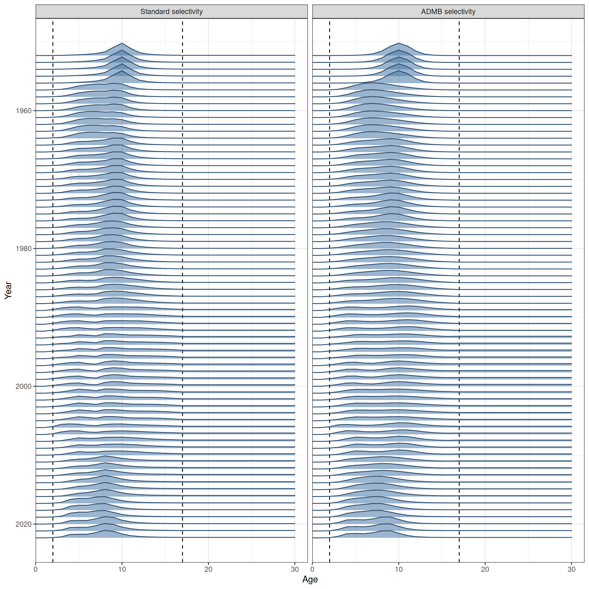
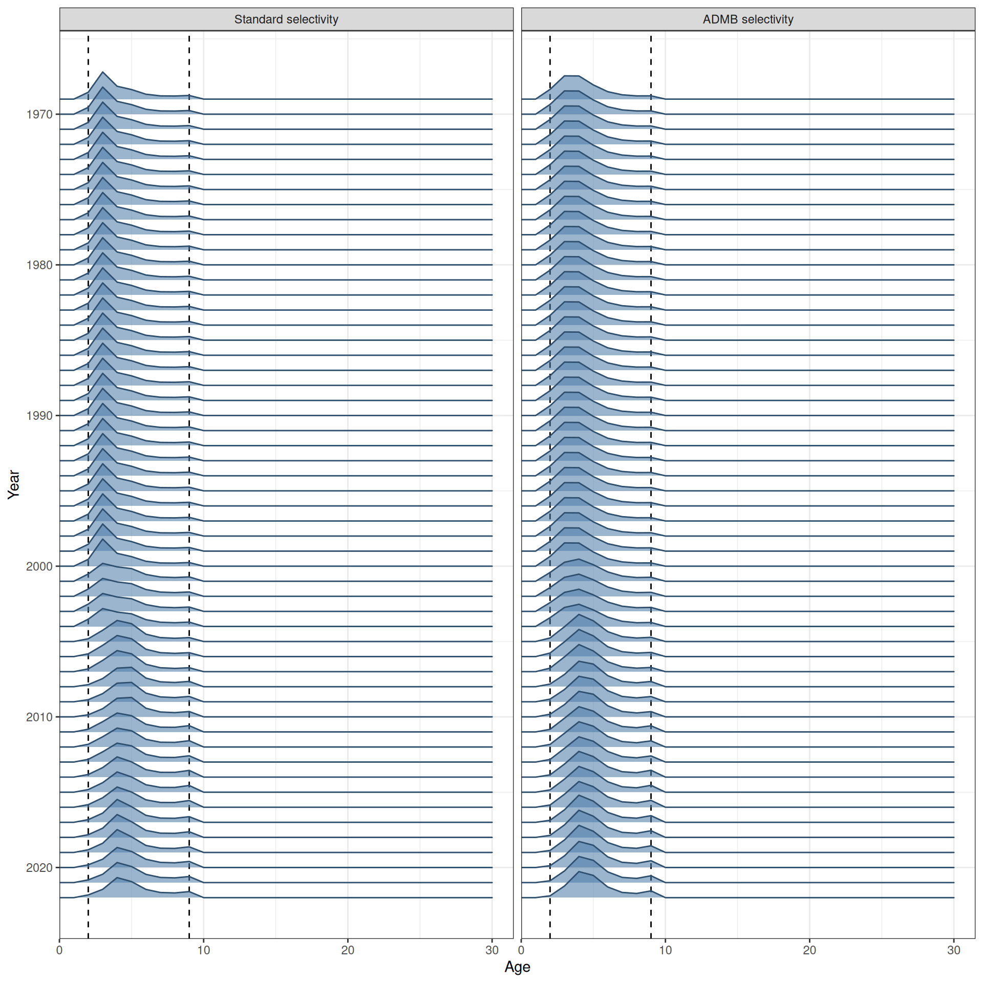
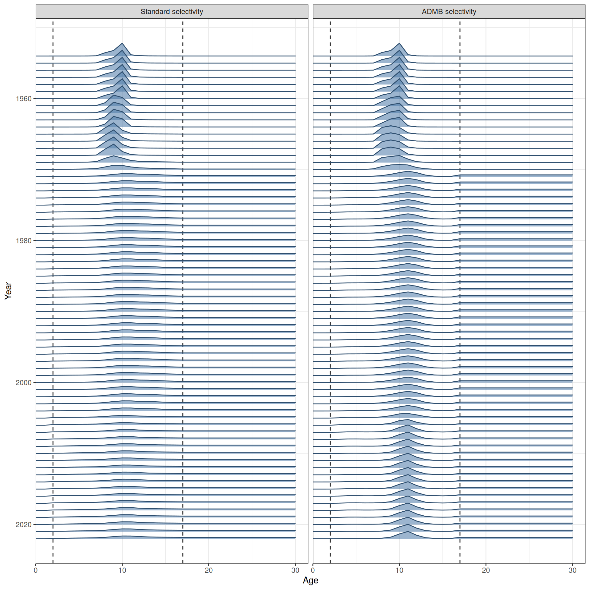
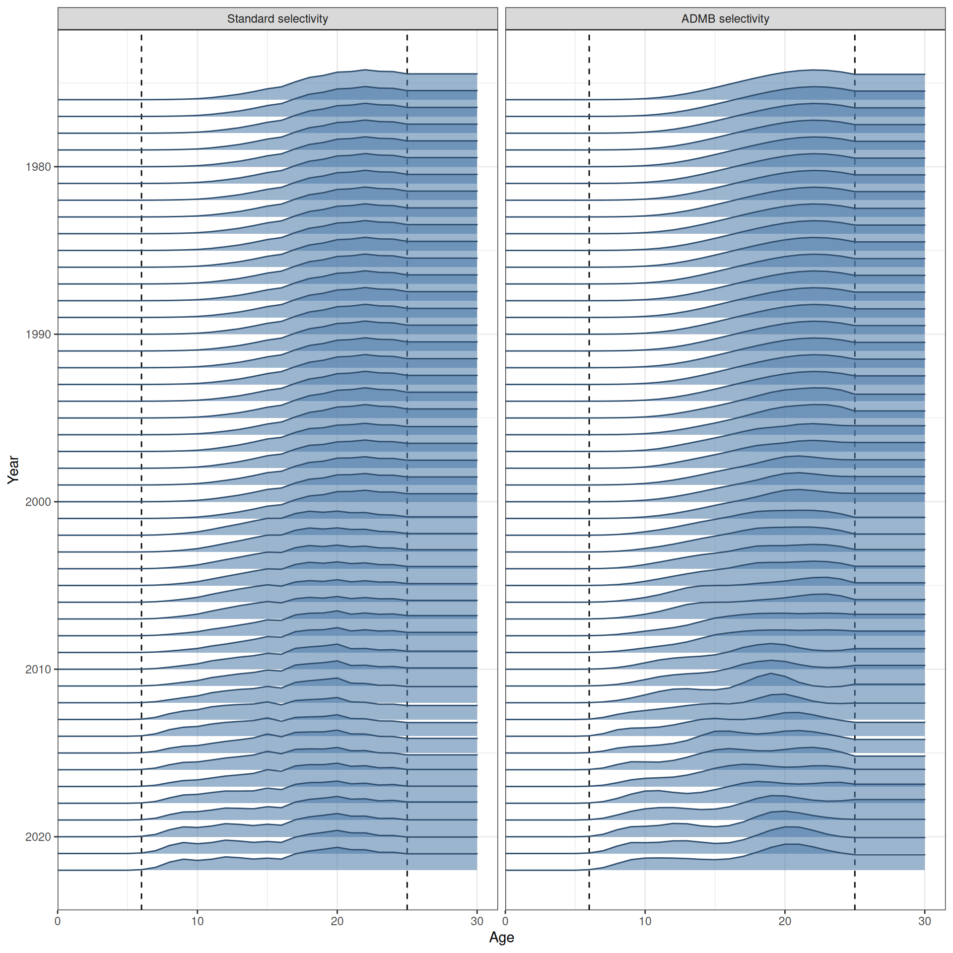
# Selectivity checks
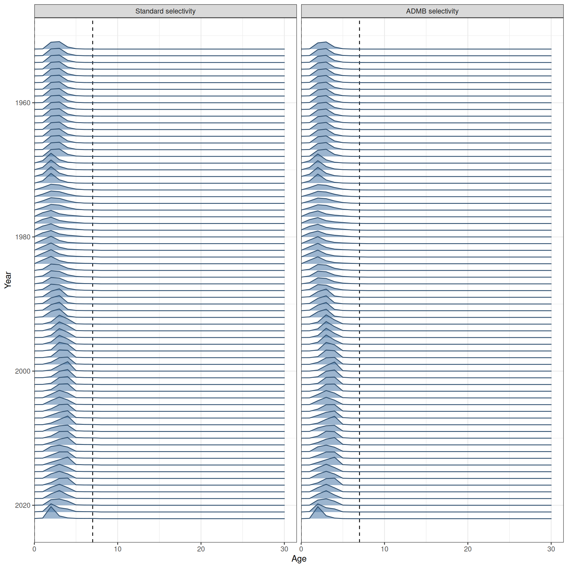
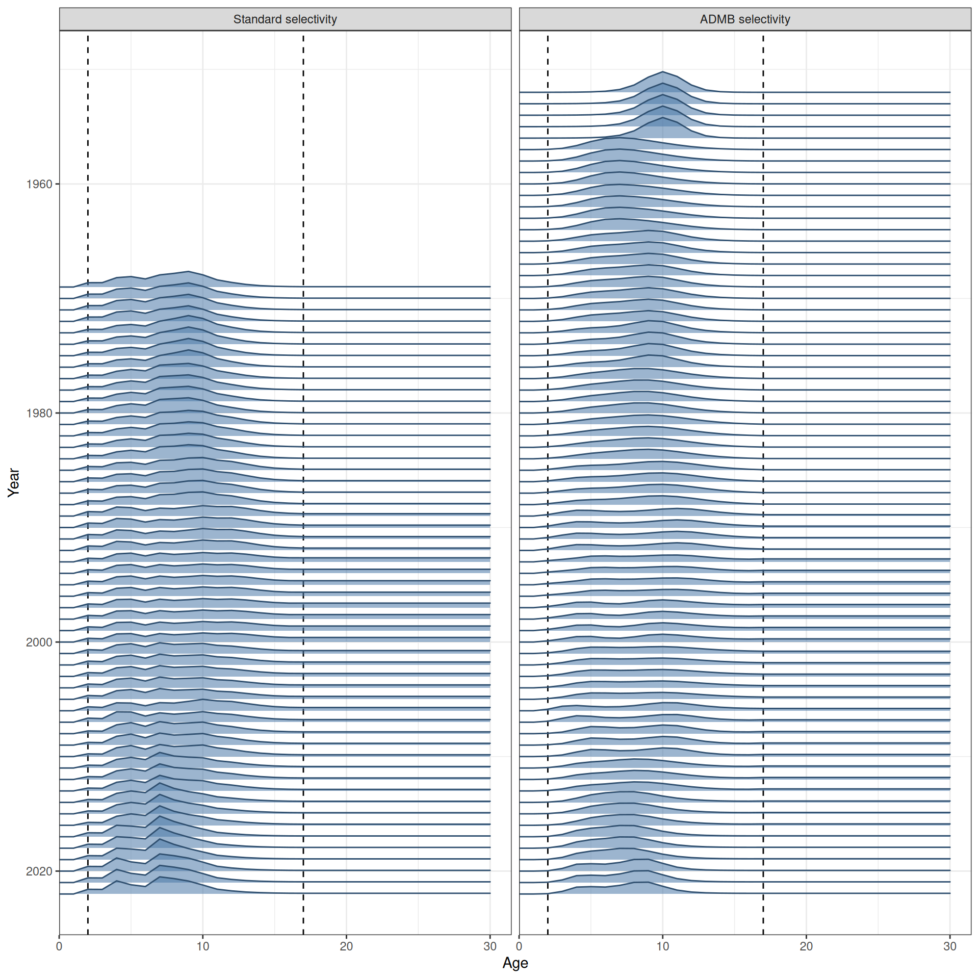
The selectivity checks compare the fitted standard selectivity model with the
ADMB-selectivity model using the reported selectivity-at-age arrays. Each figure
uses model columns so the two fitted selectivity surfaces can be compared
directly for the same fleet and years.
```{r}
#| label: selectivity-comparison-helpers
#| echo: true
#| message: false
#| warning: false
selectivity_fleets <- c("LL1", "LL2", "LL3", "LL4", "Indonesian", "Australian", "CPUE")
selectivity_model_levels <- c(
  "Standard selectivity",
  "ADMB selectivity",
  "Standard (3x age N)"
)

pad_vector <- function(x, n, fill = NA_real_) {
  c(x, rep(fill, max(0, n - length(x))))[seq_len(n)]
}

selectivity_first_years <- function(data, n_fleet) {
  cpue_first_year <- if (length(data$cpue_years) > 0) {
    data$cpue_years[1] + data$first_yr - 1
  } else {
    data$first_yr
  }
  pad_vector(c(data$first_yr_catch_f, cpue_first_year), n_fleet, fill = data$first_yr)
}

collect_selectivity <- function(data, object, model, fisheries = selectivity_fleets) {
  sel <- object$report(object$env$last.par.best)$sel_fya
  n_fleet <- dim(sel)[1]
  n_year <- dim(sel)[2]
  n_age <- dim(sel)[3]
  fleet_names <- selectivity_fleets[seq_len(n_fleet)]
  years <- seq.int(data$first_yr, length.out = n_year)
  ages <- seq.int(data$min_age, length.out = n_age)
  first_year <- selectivity_first_years(data, n_fleet)
  removal <- pad_vector(data$removal_switch_f, n_fleet, fill = 0)

  reshape2::melt(sel) |>
    as_tibble() |>
    transmute(
      model = factor(model, levels = selectivity_model_levels),
      fishery = factor(fleet_names[.data$Var1], levels = selectivity_fleets),
      year = years[.data$Var2],
      age = ages[.data$Var3],
      first_year = first_year[.data$Var1],
      removal = removal[.data$Var1],
      value = .data$value
    ) |>
    filter(
      .data$fishery %in% fisheries,
      .data$year >= .data$first_year
    )
}

collect_selectivity_ranges <- function(data, model, fisheries = selectivity_fleets) {
  n_fleet <- length(selectivity_fleets)
  tibble(
    model = factor(model, levels = selectivity_model_levels),
    fishery = factor(selectivity_fleets, levels = selectivity_fleets),
    min_age = pad_vector(data$sel_min_age_f, n_fleet),
    max_age = pad_vector(data$sel_max_age_f, n_fleet),
    removal = pad_vector(data$removal_switch_f, n_fleet, fill = 0)
  ) |>
    filter(.data$fishery %in% fisheries)
}

selectivity_comparison <- bind_rows(
  collect_selectivity(default_fit$data, default_obj, "Standard selectivity"),
  collect_selectivity(data, obj, "ADMB selectivity")
)

selectivity_ranges <- bind_rows(
  collect_selectivity_ranges(default_fit$data, "Standard selectivity"),
  collect_selectivity_ranges(data, "ADMB selectivity")
)

plot_selectivity_data <- function(df, ranges, years = NULL) {
  if (!is.null(years)) {
    df <- df |> filter(.data$year %in% years)
  }

  ggplot(
    df,
    aes(
      x = .data$age,
      y = .data$year,
      height = .data$value,
      group = interaction(.data$model, .data$year)
    )
  ) +
    geom_vline(data = ranges, aes(xintercept = .data$min_age), linetype = "dashed") +
    geom_vline(data = ranges, aes(xintercept = .data$max_age), linetype = "dashed") +
    ggridges::geom_density_ridges(
      stat = "identity",
      fill = "#4C78A8",
      colour = "#2F4F6F",
      alpha = 0.55,
      rel_min_height = 0
    ) +
    facet_grid(. ~ .data$model) +
    labs(x = "Age", y = "Year") +
    scale_x_continuous(limits = c(0, NA), expand = expansion(mult = c(0, 0.05))) +
    scale_y_reverse(breaks = scales::pretty_breaks()) +
    theme(legend.position = "none")
}

plot_selectivity_comparison <- function(fishery_name, years = NULL) {
  df <- selectivity_comparison |>
    filter(.data$fishery == .env$fishery_name)
  ranges <- selectivity_ranges |>
    filter(.data$fishery == .env$fishery_name)

  plot_selectivity_data(df, ranges, years = years)
}
```
```{r}
#| label: fig-plot-sel-ll1
#| echo: true
#| message: false
#| fig-height: 10
#| fig-width: 10
#| fig-cap: Side-by-side comparison of fitted selectivity at age by year for the LL1 fleet.
yrs <- data$first_yr_catch_f[1]:data$last_yr
plot_selectivity_comparison("LL1", years = yrs)
```
```{r}
#| label: fig-plot-sel-ll2
#| echo: true
#| message: false
#| fig-height: 10
#| fig-width: 10
#| fig-cap: Side-by-side comparison of fitted selectivity at age by year for the LL2 fleet.
yrs <- data$first_yr_catch_f[2]:data$last_yr
plot_selectivity_comparison("LL2", years = yrs)
```
```{r}
#| label: fig-plot-sel-ll3
#| echo: true
#| message: false
#| fig-height: 10
#| fig-width: 10
#| fig-cap: Side-by-side comparison of fitted selectivity at age by year for the LL3 fleet.
yrs <- data$first_yr_catch_f[3]:data$last_yr
plot_selectivity_comparison("LL3", years = yrs)
```
```{r}
#| label: fig-plot-sel-indo
#| echo: true
#| message: false
#| fig-height: 10
#| fig-width: 10
#| fig-cap: Side-by-side comparison of fitted selectivity at age by year for the Indonesian fleet.
yrs <- data$first_yr_catch_f[5]:data$last_yr
plot_selectivity_comparison("Indonesian", years = yrs)
```
```{r}
#| label: fig-plot-sel-aus
#| echo: true
#| message: false
#| fig-height: 10
#| fig-width: 10
#| fig-cap: Side-by-side comparison of fitted selectivity at age by year for the Australian fleet.
yrs <- data$first_yr_catch_f[6]:data$last_yr
plot_selectivity_comparison("Australian", years = yrs)
```
```{r}
#| label: fig-plot-sel-cpue
#| echo: true
#| message: false
#| fig-height: 10
#| fig-width: 10
#| fig-cap: Side-by-side comparison of fitted selectivity at age by year for the CPUE index.
yrs <- data$first_yr_catch_f[1]:data$last_yr
plot_selectivity_comparison("CPUE", years = yrs)
```
# Model checks
```{r}
#| label: fig-cpue-fit
#| echo: true
#| message: false
#| fig-cap: Model fits to CPUE.
set.seed(20260730)
plot_cpue(data = data, object = obj, nsim = 10)
```
```{r}
#| label: fig-plot-sbio
#| echo: true
#| message: false
#| fig-cap: Spawning biomass by year.
plot_biomass_spawning(data_list = list(data), object_list = list(obj))
```
# HSP residual diagnostics
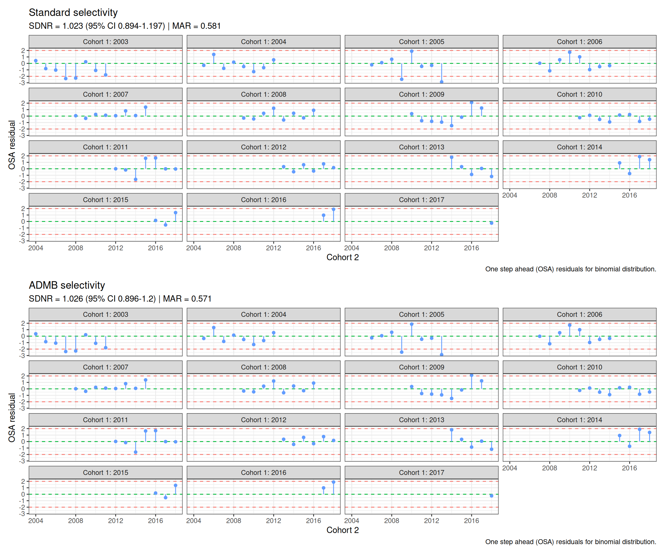
The half-sibling pair (HSP) diagnostics compare the HSP negative
log-likelihood contribution and OSA residuals under the standard and
ADMB-selectivity models. The HSP NLL in @tbl-hsp-nll is the sum of the
reported `lp_hsp` vector from each fitted model. The residual plots in
@fig-hsp-residuals use the binomial OSA residual calculation implemented in
`plot_hsps_residuals()`.
```{r}
#| label: hsp-diagnostics
#| echo: true
#| message: false
#| warning: false
model_levels <- c("Standard selectivity", "ADMB selectivity")

collect_hsp_residual_plot <- function(data, object, model_label) {
  p <- NULL
  invisible(capture.output(p <- plot_hsps_residuals(data, object)))
  list(
    plot = p + labs(title = model_label),
    residuals = as_tibble(p$data) |>
      mutate(model = factor(model_label, levels = model_levels))
  )
}

summarise_hsp_nll <- function(object, model_label) {
  rep <- object$report(object$env$last.par.best)
  tibble(
    model = factor(model_label, levels = model_levels),
    n_hsp = length(rep$lp_hsp),
    hsp_nll = sum(rep$lp_hsp)
  )
}

hsp_diagnostics <- list(
  collect_hsp_residual_plot(default_fit$data, default_obj, "Standard selectivity"),
  collect_hsp_residual_plot(data, obj, "ADMB selectivity")
)

hsp_residuals <- bind_rows(lapply(hsp_diagnostics, `[[`, "residuals"))

hsp_summary <- bind_rows(
  summarise_hsp_nll(default_obj, "Standard selectivity"),
  summarise_hsp_nll(obj, "ADMB selectivity")
) |>
  left_join(
    hsp_residuals |>
      group_by(.data$model) |>
      summarise(
        sdnr = sd(.data$resid, na.rm = TRUE),
        mar = mar(.data$resid),
        max_abs_resid = max(abs(.data$resid)),
        .groups = "drop"
      ),
    by = "model"
  )

hsp_residual_plot <- patchwork::wrap_plots(
  lapply(hsp_diagnostics, `[[`, "plot"),
  ncol = 1
)
```
```{r}
#| label: tbl-hsp-nll
#| echo: false
#| tbl-cap: "HSP negative log-likelihood and OSA residual summaries by model."
hsp_summary |>
mutate(
hsp_nll = round(.data$hsp_nll, 3),
sdnr = round(.data$sdnr, 3),
mar = round(.data$mar, 3),
max_abs_resid = round(.data$max_abs_resid, 3)
) |>
knitr::kable()
```
The HSP residual summaries in @tbl-hsp-nll provide a check on residual scale
and outlying observations, while @fig-hsp-residuals shows the residual pattern
by first cohort year and second cohort year for each model.
```{r}
#| label: fig-hsp-residuals
#| echo: true
#| message: false
#| warning: false
#| fig-width: 12
#| fig-height: 10
#| fig-cap: HSP OSA residual plots for the standard and ADMB-selectivity models.
hsp_residual_plot
```
# M10 comparison
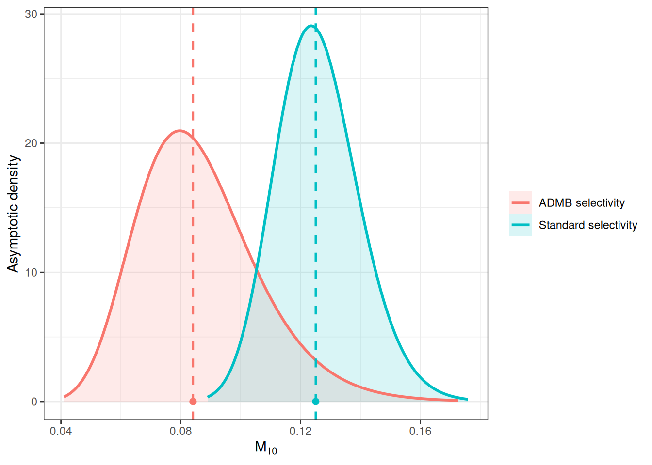
Compare the estimate of natural mortality at age 10 under the standard
selectivity implementation and the newly implemented ADMB selectivity. In this
comparison, `par_log_m10` is removed from the map so it is estimated in both
cases. Each case starts from the corresponding optimized fixed-`M10` fit, then
is re-optimized with the same bounds and control settings used above. The
asymptotic distribution is calculated on the log scale from the inverse Hessian
at the fitted mode and transformed back to `M10` for plotting.
```{r}
#| label: fit-m10-cases
#| echo: true
#| message: false
#| warning: false
update_parameters_from_fit <- function(parameters, object) {
  fitted <- object$env$parList(object$env$last.par.best)
  for (nm in intersect(names(parameters), names(fitted))) {
    parameters[[nm]] <- fitted[[nm]]
  }
  parameters
}

fit_m10_case <- function(label, model_fun, data, parameters, map, n_passes = 3) {
  map$par_log_m10 <- NULL
  case_obj <- MakeADFun(
    func = cmb(model_fun, data),
    parameters = parameters,
    map = map,
    silent = TRUE
  )
  case_bounds <- get_bounds(case_obj, parameters = parameters)
  cache_name <- paste0("m10_", gsub("[^A-Za-z0-9]+", "_", tolower(label)))
  case_opt <- run_or_load_nlminb(
    cache_name = cache_name,
    object = case_obj,
    bounds = case_bounds,
    control = control,
    n_passes = n_passes
  )
  case_obj$par <- case_opt$par
  case_obj$env$last.par.best <- case_opt$par
  case_obj$fn(case_opt$par)
  case_obj$opt <- case_opt
  case_obj$case <- label
  case_obj
}

summarise_m10_case <- function(object) {
  hessian <- object$he(object$env$last.par.best)
  covariance <- tryCatch(
    solve(hessian),
    error = function(e) MASS::ginv(hessian)
  )
  i <- match("par_log_m10", names(object$env$last.par.best))
  log_m10 <- object$env$last.par.best[i]
  se_log_m10 <- sqrt(covariance[i, i])
  if (!is.finite(se_log_m10) || se_log_m10 <= 0) {
    stop(
      "The asymptotic standard error for par_log_m10 is not positive and finite.",
      call. = FALSE
    )
  }
  tibble(
    case = object$case,
    m10_mode = exp(log_m10),
    log_m10_mode = log_m10,
    se_log_m10 = se_log_m10,
    convergence = object$opt$convergence,
    objective = object$opt$objective,
    max_gradient = max(abs(object$gr(object$env$last.par.best)))
  )
}

standard_m10_obj <- fit_m10_case(
  label = "Standard selectivity",
  model_fun = sbt_model,
  data = default_fit$data,
  parameters = update_parameters_from_fit(default_fit$parameters, default_obj),
  map = default_fit$map
)

admb_m10_obj <- fit_m10_case(
  label = "ADMB selectivity",
  model_fun = sbt_model_admb_selectivity,
  data = data,
  parameters = update_parameters_from_fit(parameters, obj),
  map = map
)

m10_summary <- bind_rows(
  summarise_m10_case(standard_m10_obj),
  summarise_m10_case(admb_m10_obj)
)
```
```{r}
#| label: tbl-m10-summary
#| echo: false
#| tbl-cap: "Mode and asymptotic uncertainty for estimated natural mortality at age 10."
m10_summary |>
mutate(
m10_mode = round(m10_mode, 4),
log_m10_mode = round(log_m10_mode, 3),
se_log_m10 = round(se_log_m10, 3),
objective = round(objective, 3),
max_gradient = signif(max_gradient, 3)
) |>
knitr::kable()
```
The like-for-like estimates in @tbl-m10-summary give `M10` modes of
`r sprintf("%.3f", m10_summary$m10_mode[m10_summary$case == "Standard selectivity"])`
for the standard-selectivity model and
`r sprintf("%.3f", m10_summary$m10_mode[m10_summary$case == "ADMB selectivity"])`
for the ADMB-selectivity model. Their corresponding asymptotic log-scale
standard errors are
`r sprintf("%.3f", m10_summary$se_log_m10[m10_summary$case == "Standard selectivity"])`
and
`r sprintf("%.3f", m10_summary$se_log_m10[m10_summary$case == "ADMB selectivity"])`.
The density curves in @fig-m10-density are drawn only over each model's central
99.8% asymptotic range, rather than being extrapolated across the full combined
x-axis.
```{r}
#| label: fig-m10-density
#| echo: true
#| message: false
#| fig-cap: Mode and asymptotic density for natural mortality at age 10.
m10_density <- m10_summary |>
  rowwise() |>
  reframe(
    case = case,
    m10 = seq(
      max(1e-6, qlnorm(0.001, log_m10_mode, se_log_m10)),
      qlnorm(0.999, log_m10_mode, se_log_m10),
      length.out = 500
    ),
    density = dlnorm(m10, log_m10_mode, se_log_m10)
  )

ggplot(m10_density, aes(x = m10, y = density, color = case, fill = case)) +
  geom_area(alpha = 0.15, position = "identity", linewidth = 0) +
  geom_line(linewidth = 1) +
  geom_vline(
    data = m10_summary,
    aes(xintercept = m10_mode, color = case),
    linetype = "dashed",
    linewidth = 0.8,
    show.legend = FALSE
  ) +
  geom_point(
    data = m10_summary,
    aes(x = m10_mode, y = 0, color = case),
    size = 2,
    show.legend = FALSE
  ) +
  labs(x = expression(M[10]), y = "Asymptotic density", color = NULL, fill = NULL)
```
# OSA residuals for composition fits
The OSA diagnostics follow the multinomial composition-data residual approach
described by @StewartMonnahan2025 and implemented in `afscOSA`. When `afscOSA`
is available it is used directly; otherwise the same sequential multinomial
randomized quantile residual calculation is evaluated in this vignette. The
current SBT likelihoods use KL-divergence weights for age and length
compositions, so these OSA plots are used as a diagnostic only. The
calculations use the model composition sample sizes as `N`, the fitted expected
proportions from each model, and the bins used by each composition likelihood.
The aggregate-fit panels are calculated as input-sample-size weighted
proportions, `sum_y N_y p_y / sum_y N_y`, separately for the observed and fitted
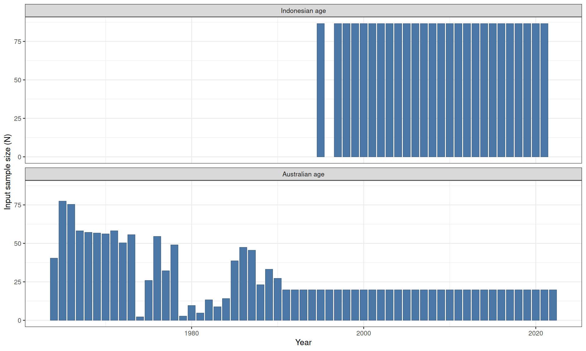
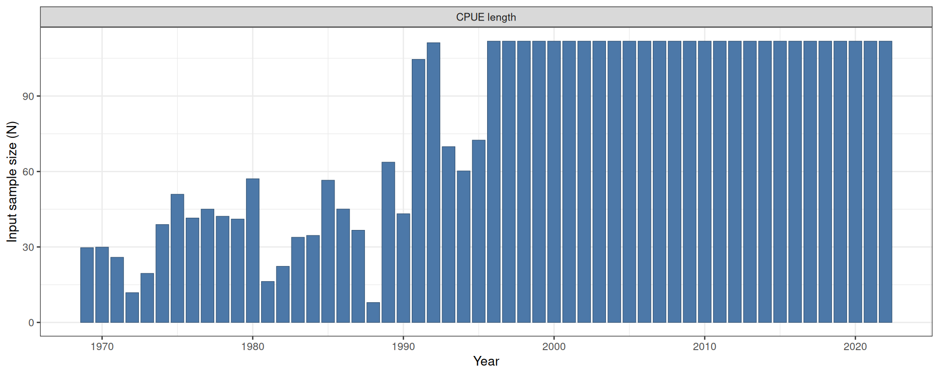
compositions. The annual sample sizes used as multinomial `N` values are shown
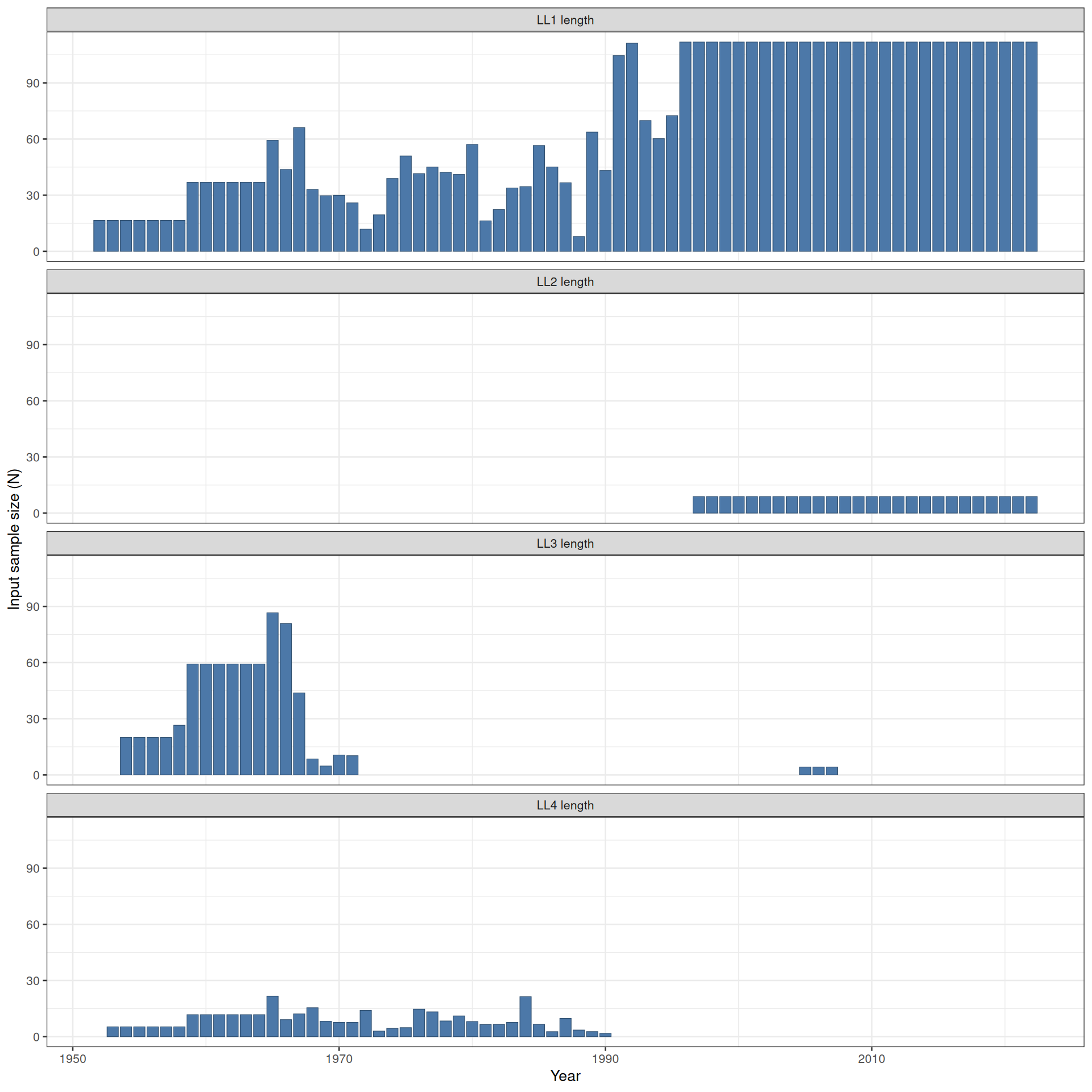
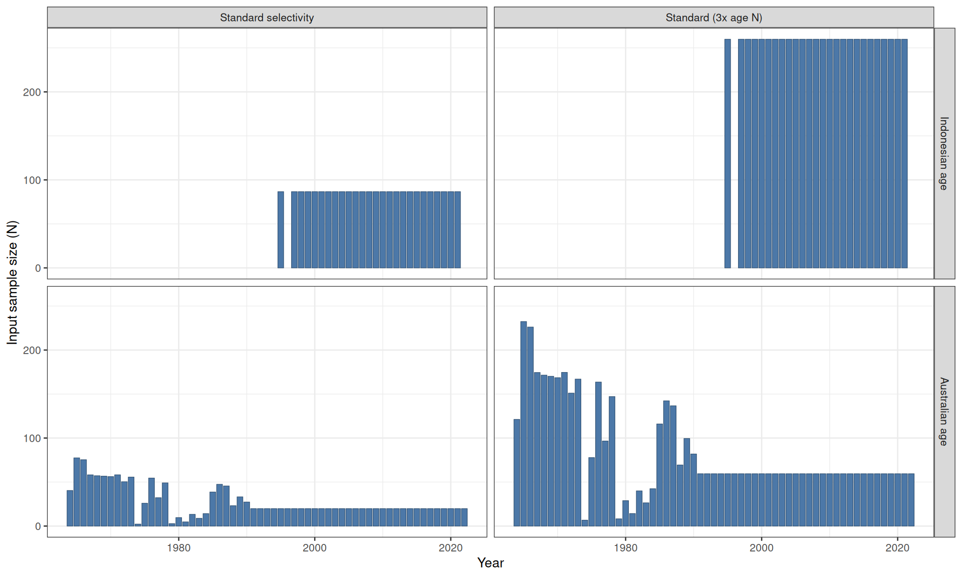
for the age-composition diagnostics in @fig-osa-age-n, the longline
length-composition diagnostics in @fig-osa-lf-n, and the CPUE
length-composition diagnostics in @fig-osa-cpue-lf-n. These sample sizes are
shown once because the same input composition data are used for both models.
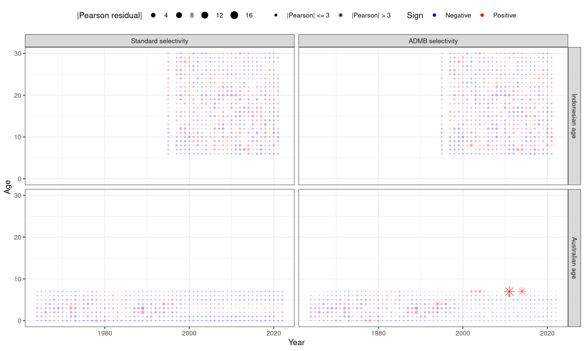
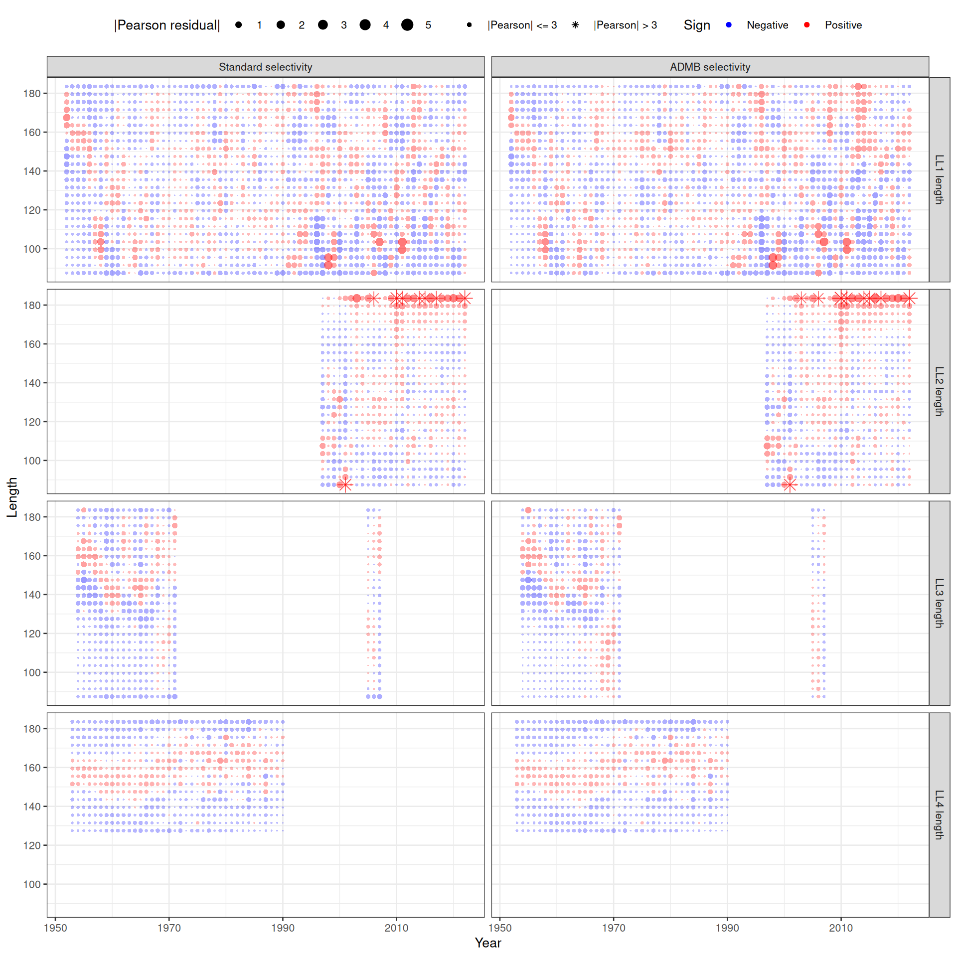
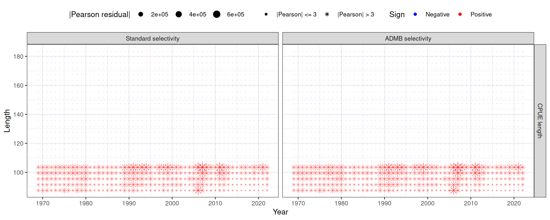
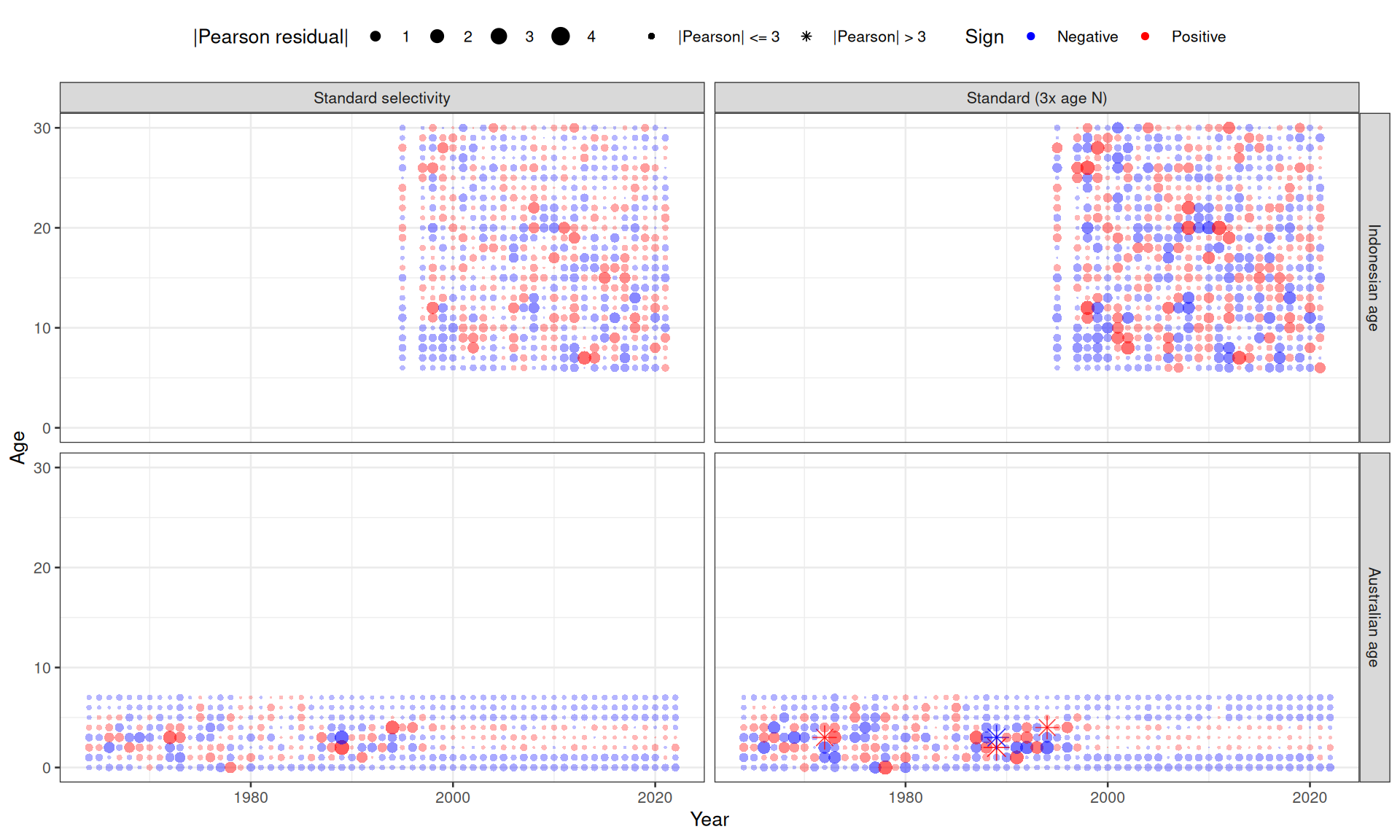
Pearson residual bubble diagnostics are shown in @fig-osa-age-pearson,
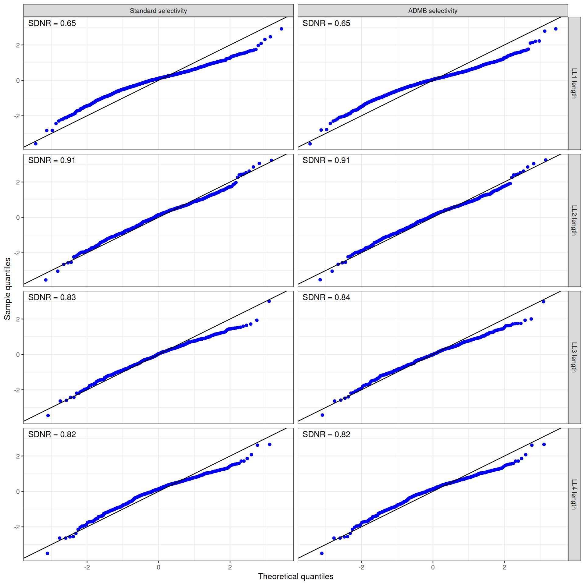
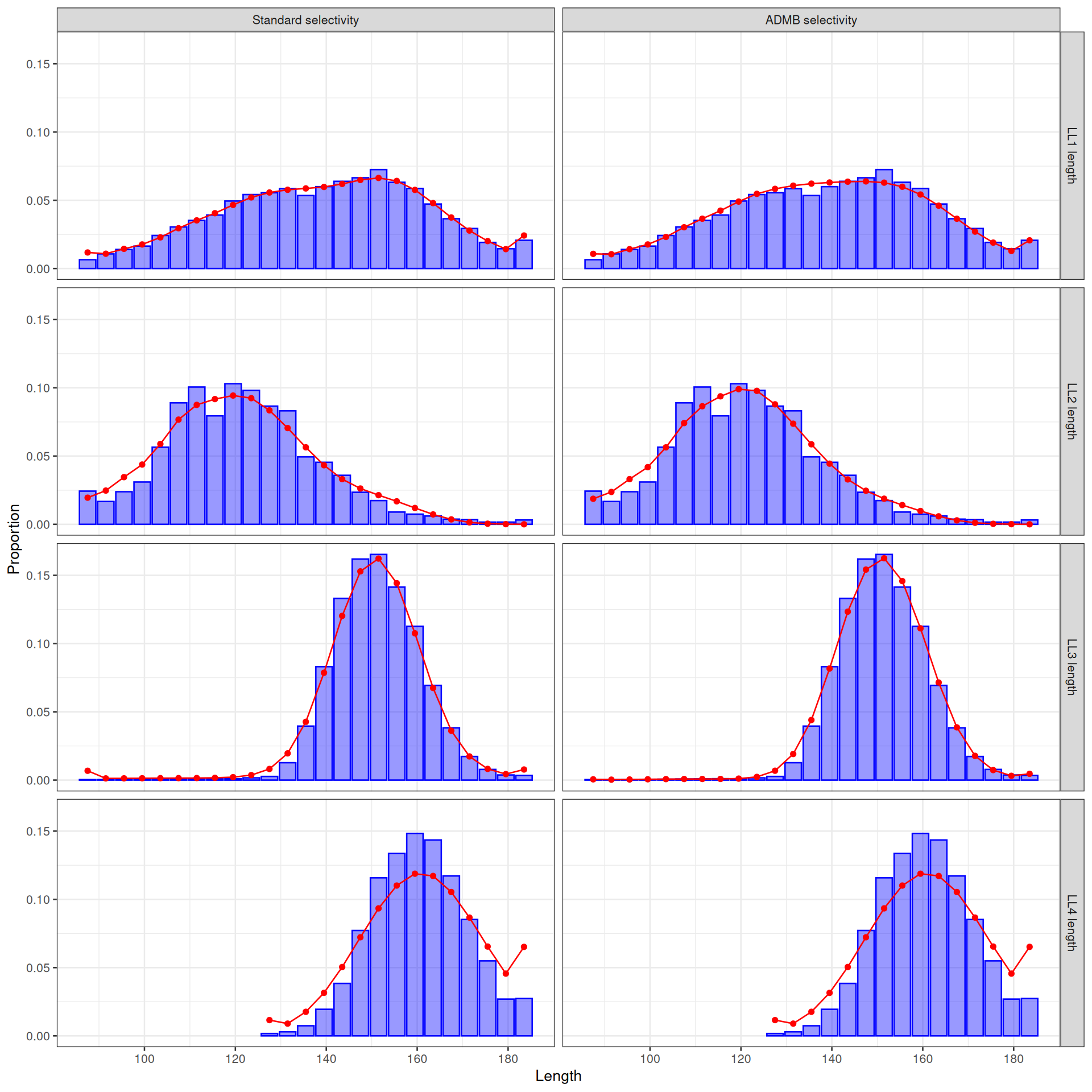
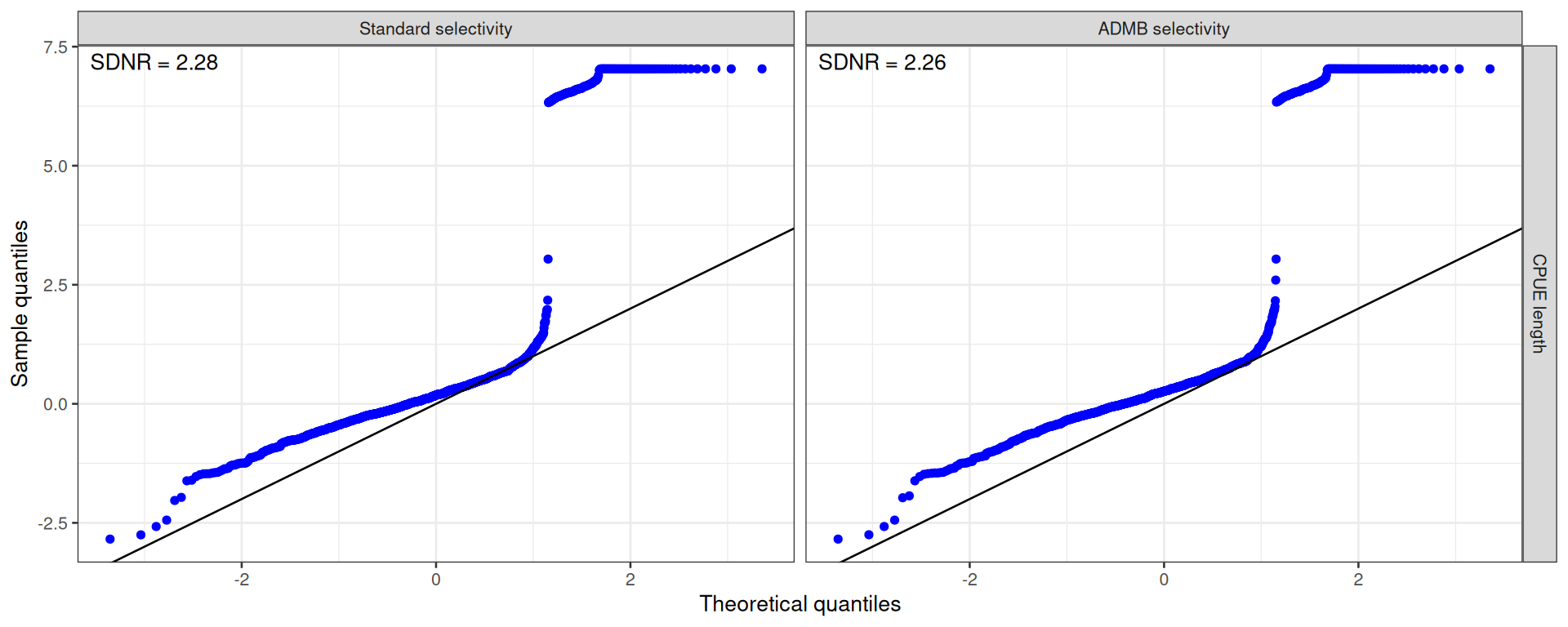
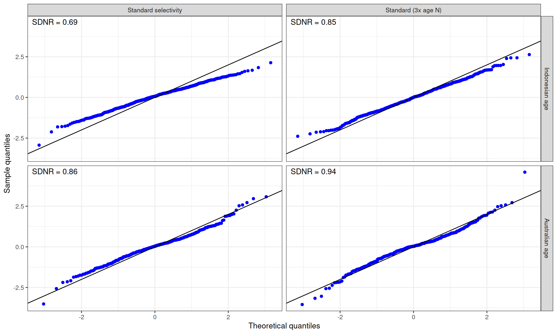
@fig-osa-lf-pearson, and @fig-osa-cpue-lf-pearson. The residual Q-Q and
aggregate-fit diagnostics are shown in @fig-osa-age-qq and @fig-osa-age-agg for
age compositions, @fig-osa-lf-qq and @fig-osa-lf-agg for longline length
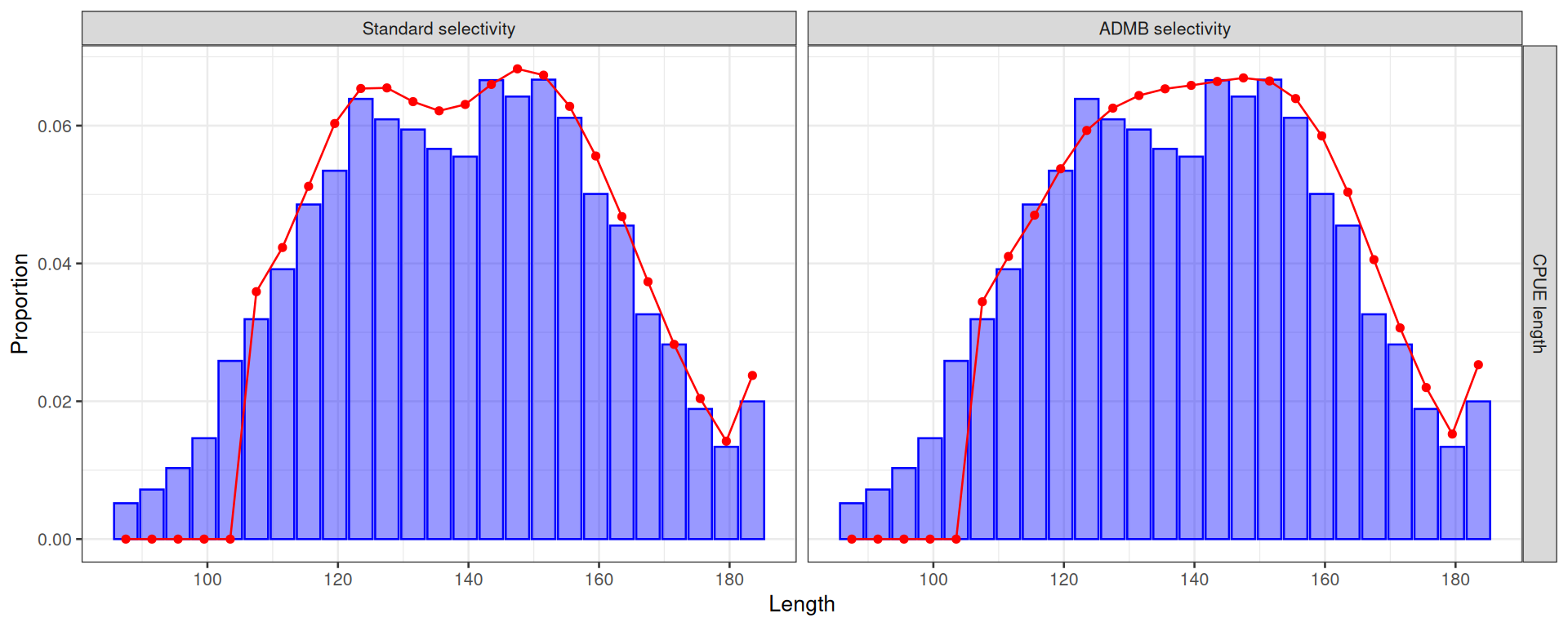
compositions, and @fig-osa-cpue-lf-qq and @fig-osa-cpue-lf-agg for CPUE length
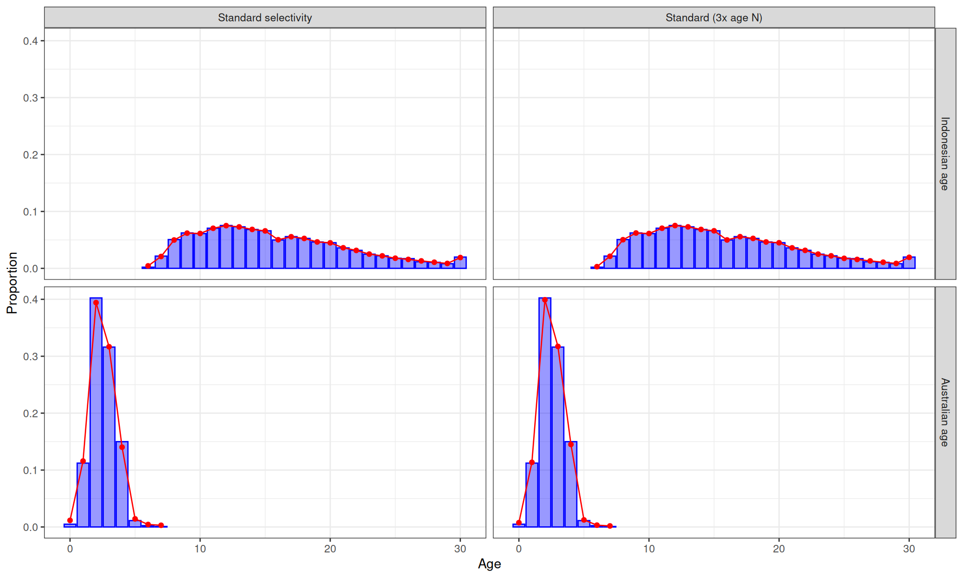
compositions. The residual diagnostic figures are faceted with fleet rows and
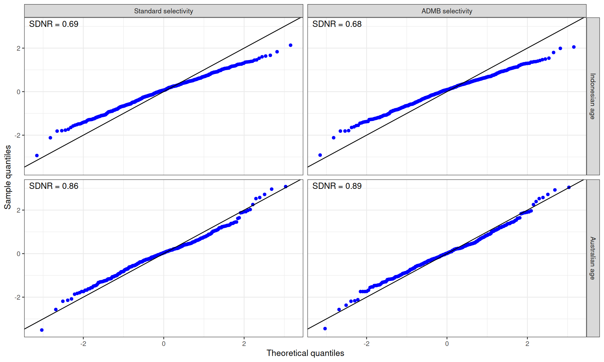
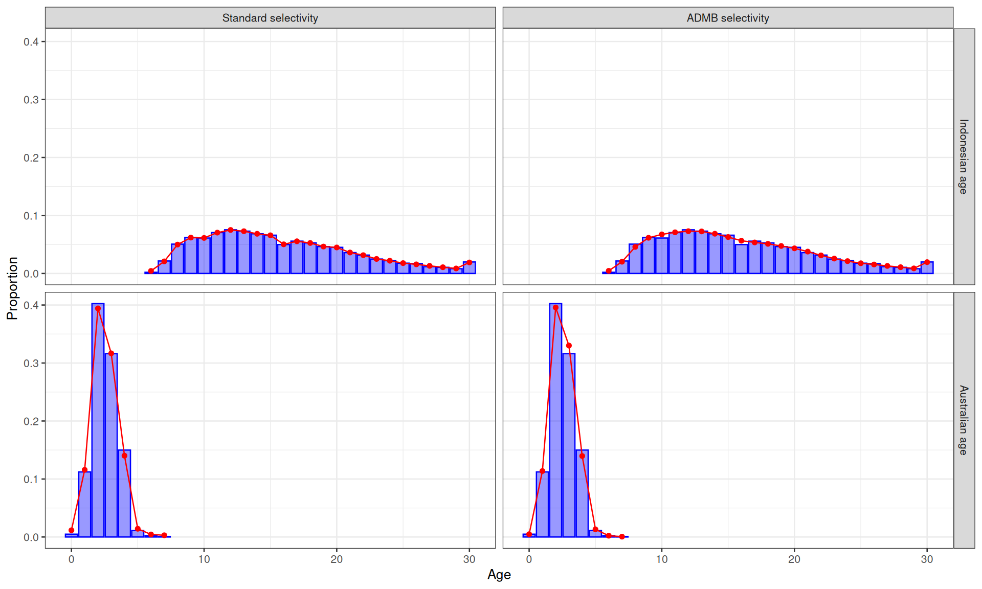
model columns.
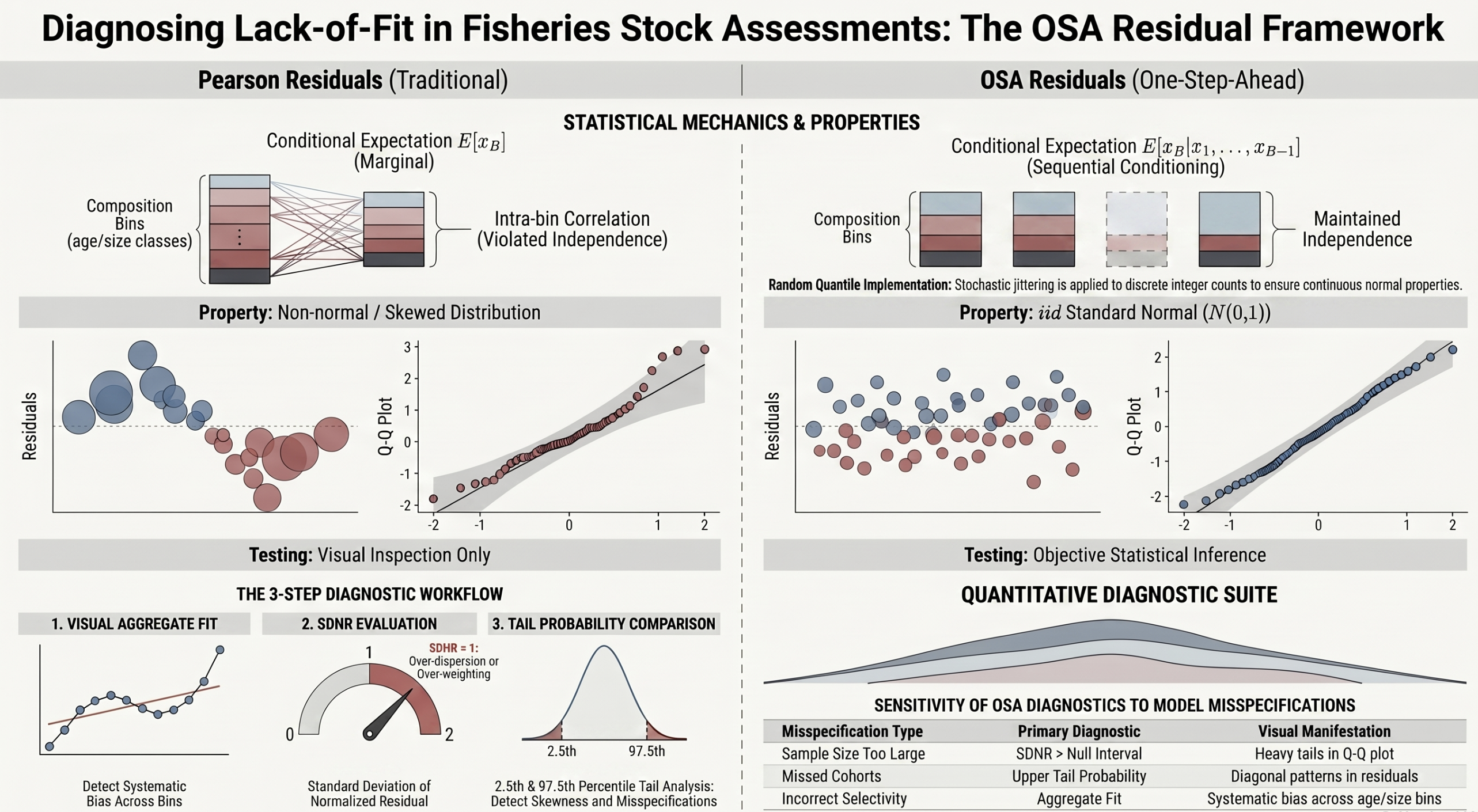{#fig-osa-framework fig-alt="Infographic comparing traditional Pearson residual diagnostics with one-step-ahead residual diagnostics for stock-assessment composition data. Pearson residuals use marginal expectations and can show correlated, skewed residuals, while OSA residuals use sequential conditioning and randomized quantile residuals to support standard-normal Q-Q and SDNR diagnostics."}
The OSA residual framework summarized in @fig-osa-framework is used here
because composition residuals are not independent normal observations in their
raw form. Traditional Pearson residual bubble plots remain useful for locating
bins, years, or fleets with local misfit, but they are primarily a visual
diagnostic and can inherit the correlation and skewness imposed by the
multinomial composition constraint. OSA residuals instead evaluate each
composition bin sequentially, conditional on the previous bins in that
observation. With the randomized quantile step for discrete counts, a correctly
specified multinomial diagnostic model should produce residuals that are
approximately independent standard normal values. This makes the Q-Q plots and
SDNR summaries interpretable as formal checks of tail behavior and residual
scale, while the aggregate-fit and Pearson panels show where any lack of fit
occurs in the observed composition data.
```{r}
#| label: osa-helpers
#| echo: true
#| message: false
#| warning: false
normalise_composition <- function(x, eps = 1e-12) {
  x <- as.matrix(x)
  x[!is.finite(x)] <- 0
  x <- pmax(x, eps)
  x / rowSums(x)
}

multinomial_osa_residuals <- function(counts, probs, eps = 1e-12, seed = 99801) {
  counts <- as.matrix(counts)
  probs <- normalise_composition(probs, eps = eps)
  n_bins <- ncol(counts)
  out <- matrix(NA_real_, nrow = nrow(counts), ncol = max(n_bins - 1, 0))
  if (n_bins <= 1) return(out)

  old_seed <- if (exists(".Random.seed", envir = .GlobalEnv, inherits = FALSE)) {
    get(".Random.seed", envir = .GlobalEnv)
  } else {
    NULL
  }
  on.exit({
    if (is.null(old_seed)) {
      rm(".Random.seed", envir = .GlobalEnv)
    } else {
      assign(".Random.seed", old_seed, envir = .GlobalEnv)
    }
  }, add = TRUE)
  set.seed(seed)

  for (i in seq_len(nrow(counts))) {
    x <- round(counts[i, ])
    p <- probs[i, ]
    n_remaining <- sum(x)
    p_remaining <- sum(p)

    for (j in seq_len(n_bins - 1)) {
      if (n_remaining <= 0 || p_remaining <= eps) next
      prob_j <- pmin(pmax(p[j] / p_remaining, eps), 1 - eps)
      x_j <- pmin(pmax(x[j], 0), n_remaining)
      lower <- if (x_j <= 0) 0 else pbinom(x_j - 1, n_remaining, prob_j)
      mass <- dbinom(x_j, n_remaining, prob_j)
      u <- lower + runif(1) * mass
      out[i, j] <- qnorm(pmin(pmax(u, eps), 1 - eps))
      n_remaining <- n_remaining - x_j
      p_remaining <- p_remaining - p[j]
    }
  }

  out
}

run_local_osa <- function(obs, exp, N, fleet, index, years, index_label) {
  counts <- round(sweep(obs, 1, N, `*`), 0)
  probs <- normalise_composition(exp)
  res_mat <- multinomial_osa_residuals(counts, probs)
  dimnames(res_mat) <- list(year = years, index = index[seq_len(ncol(res_mat))])
  res <- reshape2::melt(res_mat, value.name = "resid") |>
    as_tibble() |>
    mutate(
      fleet = fleet,
      index_label = index_label
    ) |>
    relocate(.data$fleet, .data$index_label, .before = .data$year)

  list(
    res = res,
    agg = data.frame(
      fleet = fleet,
      index_label = index_label,
      index = index,
      obs = colSums(counts) / sum(counts),
      exp = colSums(probs) / sum(probs)
    )
  )
}

run_osa_values <- function(obs, exp, N, fleet, index, years, index_label) {
  if (requireNamespace("afscOSA", quietly = TRUE) &&
      !identical(tolower(Sys.getenv("SBT_USE_LOCAL_OSA")), "true")) {
    out <- tryCatch(
      afscOSA::run_osa(
        obs = obs,
        exp = exp,
        N = N,
        fleet = fleet,
        index = index,
        years = years,
        index_label = index_label
      ),
      error = function(e) NULL
    )
    if (!is.null(out) && is.data.frame(out$res)) return(out)
  }

  run_local_osa(
    obs = obs,
    exp = exp,
    N = N,
    fleet = fleet,
    index = index,
    years = years,
    index_label = index_label
  )
}

run_osa_block <- function(obs, exp, N, fleet, index, years, index_label) {
  valid <- is.finite(N) & N > 0 & rowSums(obs) > 0 & rowSums(exp) > 0
  obs <- normalise_composition(obs[valid, , drop = FALSE])
  exp <- normalise_composition(exp[valid, , drop = FALSE])
  N <- N[valid]
  years <- years[valid]
  out <- run_osa_values(
    obs = obs,
    exp = exp,
    N = N,
    fleet = fleet,
    index = index,
    years = years,
    index_label = index_label
  )
  out$agg <- data.frame(
    fleet = fleet,
    index_label = index_label,
    index = index,
    obs = colSums(sweep(obs, 1, N, `*`)) / sum(N),
    exp = colSums(sweep(exp, 1, N, `*`)) / sum(N)
  )
  out$sample_size <- data.frame(
    fleet = fleet,
    index_label = index_label,
    year = years,
    N = N
  )
  obs_count <- sweep(obs, 1, N, `*`)
  exp_count <- sweep(exp, 1, N, `*`)
  pearson <- (obs_count - exp_count) /
    sqrt(pmax(exp_count * pmax(1 - exp, 1e-12), 1e-12))
  out$pearson <- data.frame(
    fleet = fleet,
    index_label = index_label,
    year = rep(years, times = length(index)),
    index = rep(index, each = length(years)),
    resid = as.vector(pearson)
  )
  out
}

make_age_osa <- function(data, object, model_label) {
  rep <- object$report(object$env$last.par.best)
  fleet_names <- c(`5` = "Indonesian age", `6` = "Australian age")
  lapply(c(5, 6), function(f) {
    keep <- data$af_fishery == f & data$af_n > 0
    ages <- seq.int(unique(data$af_min_age[keep]), unique(data$af_max_age[keep]))
    cols <- ages + 1
    run_osa_block(
      obs = data$af_obs[keep, cols, drop = FALSE],
      exp = rep$af_pred[keep, cols, drop = FALSE],
      N = data$af_n[keep],
      fleet = paste(model_label, fleet_names[as.character(f)], sep = ": "),
      index = ages,
      years = data$af_year[keep] + data$first_yr - 1,
      index_label = "Age"
    )
  })
}

make_lf_osa <- function(data, object, model_label) {
  rep <- object$report(object$env$last.par.best)
  fleet_names <- c("LL1 length", "LL2 length", "LL3 length", "LL4 length")
  length_bins <- seq(87.5, by = 4, length.out = ncol(data$lf_obs))
  lapply(seq_along(fleet_names), function(f) {
    keep <- data$lf_fishery == f & data$lf_n > 0
    cols <- data$lf_minbin[f]:ncol(data$lf_obs)
    run_osa_block(
      obs = data$lf_obs[keep, cols, drop = FALSE],
      exp = rep$lf_pred[keep, cols, drop = FALSE],
      N = data$lf_n[keep],
      fleet = paste(model_label, fleet_names[f], sep = ": "),
      index = length_bins[cols],
      years = data$lf_year[keep] + data$first_yr - 1,
      index_label = "Length"
    )
  })
}

make_cpue_lf_osa <- function(data, object, model_label) {
  rep <- object$report(object$env$last.par.best)
  length_bins <- seq(87.5, by = 4, length.out = ncol(data[["cpue_lfs"]]))
  list(
    run_osa_block(
      obs = data[["cpue_lfs"]],
      exp = rep$cpue_lf_pred,
      N = data$cpue_n,
      fleet = paste(model_label, "CPUE length", sep = ": "),
      index = length_bins,
      years = data$cpue_years + data$first_yr - 1,
      index_label = "Length"
    )
  )
}

osa_outpath <- file.path(tempdir(), "sbt_admb_selectivity_osa")

osa_age <- c(
  make_age_osa(default_fit$data, default_obj, "Standard selectivity"),
  make_age_osa(data, obj, "ADMB selectivity")
)

osa_lf <- c(
  make_lf_osa(default_fit$data, default_obj, "Standard selectivity"),
  make_lf_osa(data, obj, "ADMB selectivity")
)

osa_cpue_lf <- c(
  make_cpue_lf_osa(default_fit$data, default_obj, "Standard selectivity"),
  make_cpue_lf_osa(data, obj, "ADMB selectivity")
)

osa_model_levels <- c(model_levels, "Standard (3x age N)")

parse_osa_labels <- function(x) {
  fleet_name <- sub("^[^:]+: ", "", x$fleet)
  x |>
    as_tibble() |>
    mutate(
      model = factor(
        sub(": .*", "", .data$fleet),
        levels = osa_model_levels
      ),
      fleet = factor(fleet_name, levels = unique(fleet_name))
    )
}

collect_osa_res <- function(input) {
  bind_rows(lapply(input, `[[`, "res")) |>
    filter(is.finite(.data$resid)) |>
    parse_osa_labels()
}

collect_osa_agg <- function(input) {
  bind_rows(lapply(input, `[[`, "agg")) |>
    parse_osa_labels()
}

collect_osa_sample_size <- function(input) {
  bind_rows(lapply(input, `[[`, "sample_size")) |>
    parse_osa_labels()
}

collect_osa_pearson <- function(input) {
  bind_rows(lapply(input, `[[`, "pearson")) |>
    filter(is.finite(.data$resid)) |>
    parse_osa_labels()
}

make_osa_qq <- function(input) {
  res <- collect_osa_res(input)
  sdnr <- res |>
    group_by(.data$model, .data$fleet) |>
    summarise(
      sdnr = paste0("SDNR = ", sprintf("%.2f", sd(.data$resid, na.rm = TRUE))),
      .groups = "drop"
    )

  ggplot() +
    stat_qq(data = res, aes(sample = .data$resid), color = "blue") +
    geom_abline(slope = 1, intercept = 0) +
    geom_text(
      data = sdnr,
      aes(x = -Inf, y = Inf, label = .data$sdnr),
      hjust = -0.1,
      vjust = 1.5
    ) +
    facet_grid(.data$fleet ~ .data$model) +
    labs(x = "Theoretical quantiles", y = "Sample quantiles") +
    theme_bw(base_size = 10)
}

make_osa_sample_size <- function(input) {
  sample_size <- collect_osa_sample_size(input)
  sample_size_check <- sample_size |>
    group_by(.data$fleet, .data$index_label, .data$year) |>
    summarise(n_values = n_distinct(.data$N), .groups = "drop")
  stopifnot(all(sample_size_check$n_values == 1))
  sample_size <- sample_size |>
    distinct(.data$fleet, .data$index_label, .data$year, .data$N)

  ggplot(sample_size, aes(x = .data$year, y = .data$N)) +
    geom_col(fill = "#4C78A8", color = "#2F4F6F", width = 0.85, linewidth = 0.2) +
    facet_wrap(~fleet, ncol = 1) +
    scale_y_continuous(labels = scales::label_comma()) +
    labs(x = "Year", y = "Input sample size (N)") +
    theme_bw(base_size = 10)
}

make_osa_pearson_bubble <- function(input) {
  res <- collect_osa_pearson(input) |>
    mutate(
      sign = factor(if_else(.data$resid < 0, "Negative", "Positive"),
                    levels = c("Negative", "Positive")),
      outlier = factor(
        if_else(abs(.data$resid) > 3, "|Pearson| > 3", "|Pearson| <= 3"),
        levels = c("|Pearson| <= 3", "|Pearson| > 3")
      )
    )

  ggplot(
    res,
    aes(
      x = .data$year,
      y = .data$index,
      size = abs(.data$resid),
      color = .data$sign,
      alpha = abs(.data$resid),
      shape = .data$outlier
    )
  ) +
    geom_point() +
    scale_color_manual(values = c(Negative = "blue", Positive = "red")) +
    scale_size(range = c(0.1, 4), name = "|Pearson residual|") +
    scale_alpha(range = c(0.25, 0.85), guide = "none") +
    scale_shape_manual(values = c("|Pearson| <= 3" = 16, "|Pearson| > 3" = 8), name = NULL) +
    facet_grid(.data$fleet ~ .data$model) +
    {
      if (length(unique(res$index)) < 20) {
        scale_y_continuous(breaks = sort(unique(res$index)), labels = sort(unique(res$index)))
      }
    } +
    labs(x = "Year", y = unique(res$index_label), color = "Sign") +
    guides(
      size = guide_legend(order = 1),
      shape = guide_legend(order = 2),
      color = guide_legend(order = 3)
    ) +
    theme_bw(base_size = 10) +
    theme(legend.position = "top")
}

make_osa_agg <- function(input) {
  agg <- collect_osa_agg(input)

  ggplot(data = agg) +
    geom_col(aes(x = .data$index, y = .data$obs), color = "blue", fill = "blue", alpha = 0.4) +
    geom_point(aes(x = .data$index, y = .data$exp), color = "red") +
    geom_line(aes(x = .data$index, y = .data$exp), color = "red") +
    facet_grid(.data$fleet ~ .data$model) +
    {
      if (length(unique(agg$index)) < 20) {
        scale_x_continuous(breaks = unique(agg$index), labels = unique(agg$index))
      }
    } +
    labs(x = unique(agg$index_label), y = "Proportion") +
    theme_bw(base_size = 10)
}

summarise_osa_sdnr <- function(input, composition) {
  bind_rows(lapply(input, `[[`, "res")) |>
    as_tibble() |>
    mutate(
      composition = composition,
      model = factor(
        sub(": .*", "", .data$fleet),
        levels = osa_model_levels
      ),
      fleet = sub("^[^:]+: ", "", .data$fleet)
    ) |>
    group_by(.data$composition, .data$model, .data$fleet) |>
    summarise(
      n_residuals = sum(is.finite(.data$resid)),
      sdnr = sd(.data$resid, na.rm = TRUE),
      n_abs_resid_gt_3 = sum(abs(.data$resid) > 3, na.rm = TRUE),
      max_abs_resid = max(abs(.data$resid), na.rm = TRUE),
      .groups = "drop"
    ) |>
    mutate(
      sdnr = round(.data$sdnr, 3),
      max_abs_resid = round(.data$max_abs_resid, 3)
    )
}

osa_plot_parts <- list(
  age = list(
    n = make_osa_sample_size(osa_age),
    pearson = make_osa_pearson_bubble(osa_age),
    qq = make_osa_qq(osa_age),
    aggcomp = make_osa_agg(osa_age)
  ),
  lf = list(
    n = make_osa_sample_size(osa_lf),
    pearson = make_osa_pearson_bubble(osa_lf),
    qq = make_osa_qq(osa_lf),
    aggcomp = make_osa_agg(osa_lf)
  ),
  cpue_lf = list(
    n = make_osa_sample_size(osa_cpue_lf),
    pearson = make_osa_pearson_bubble(osa_cpue_lf),
    qq = make_osa_qq(osa_cpue_lf),
    aggcomp = make_osa_agg(osa_cpue_lf)
  )
)

osa_sdnr <- bind_rows(
  summarise_osa_sdnr(osa_age, "Age composition"),
  summarise_osa_sdnr(osa_lf, "Longline length composition"),
  summarise_osa_sdnr(osa_cpue_lf, "CPUE length composition")
)
```
```{r}
#| label: tbl-osa-sdnr
#| echo: false
#| tbl-cap: "OSA SDNR diagnostics for age and length compositions under the standard and ADMB-selectivity models."
osa_sdnr |>
arrange(composition, fleet, model) |>
knitr::kable()
```
The age-composition and longline length-composition SDNR values in
@tbl-osa-sdnr are below 1, indicating residuals that are narrower than expected
under the multinomial diagnostic distribution. In contrast, the CPUE
length-composition SDNR is about 2.26--2.28 and has 157 residuals with absolute
value greater than 3 under both formulations, identifying that data set as the
clear lack-of-fit exception. The two selectivity formulations nevertheless
give very similar diagnostics: ADMB selectivity raises the Australian-age,
LL1, and LL3 SDNRs slightly; lowers the Indonesian-age, CPUE, and LL2 SDNRs
slightly; and leaves LL4 effectively unchanged. The Q-Q plots show the same
pattern: most age and longline panels have compressed tails relative to the
1:1 line, whereas the CPUE panel has substantially inflated tails. The
aggregate fits indicate that the two models produce very similar overall
composition shapes. The sample-size figures show the annual weighting used by
the multinomial OSA diagnostics and the N-weighted aggregate panels; these
inputs are shown once because the two selectivity formulations are evaluated
against the same composition data. The Pearson residual bubbles show where the
observed proportions are above or below the model expectation after scaling by
the same input sample sizes.
```{r}
#| label: fig-osa-age-n
#| echo: true
#| message: false
#| warning: false
#| fig-width: 10
#| fig-height: 6
#| fig-cap: Input sample sizes used for age-composition OSA diagnostics.
osa_plot_parts$age$n
```
```{r}
#| label: fig-osa-age-pearson
#| echo: true
#| message: false
#| warning: false
#| fig-width: 10
#| fig-height: 6
#| fig-cap: Pearson residual bubble plots for age compositions.
osa_plot_parts$age$pearson
```
```{r}
#| label: fig-osa-age-qq
#| echo: true
#| message: false
#| warning: false
#| fig-width: 10
#| fig-height: 6
#| fig-cap: OSA Q-Q plots for age compositions.
osa_plot_parts$age$qq
```
```{r}
#| label: fig-osa-age-agg
#| echo: true
#| message: false
#| warning: false
#| fig-width: 10
#| fig-height: 6
#| fig-cap: Aggregate OSA fits for age compositions.
osa_plot_parts$age$aggcomp
```
```{r}
#| label: fig-osa-lf-n
#| echo: true
#| message: false
#| warning: false
#| fig-width: 10
#| fig-height: 10
#| fig-cap: Input sample sizes used for longline length-composition OSA diagnostics.
osa_plot_parts$lf$n
```
```{r}
#| label: fig-osa-lf-pearson
#| echo: true
#| message: false
#| warning: false
#| fig-width: 10
#| fig-height: 10
#| fig-cap: Pearson residual bubble plots for longline length compositions.
osa_plot_parts$lf$pearson
```
```{r}
#| label: fig-osa-lf-qq
#| echo: true
#| message: false
#| warning: false
#| fig-width: 10
#| fig-height: 10
#| fig-cap: OSA Q-Q plots for longline length compositions.
osa_plot_parts$lf$qq
```
```{r}
#| label: fig-osa-lf-agg
#| echo: true
#| message: false
#| warning: false
#| fig-width: 10
#| fig-height: 10
#| fig-cap: Aggregate OSA fits for longline length compositions.
osa_plot_parts$lf$aggcomp
```
```{r}
#| label: fig-osa-cpue-lf-n
#| echo: true
#| message: false
#| warning: false
#| fig-width: 10
#| fig-height: 4
#| fig-cap: Input sample sizes used for CPUE length-composition OSA diagnostics.
osa_plot_parts$cpue_lf$n
```
```{r}
#| label: fig-osa-cpue-lf-pearson
#| echo: true
#| message: false
#| warning: false
#| fig-width: 10
#| fig-height: 4
#| fig-cap: Pearson residual bubble plots for CPUE length compositions.
osa_plot_parts$cpue_lf$pearson
```
```{r}
#| label: fig-osa-cpue-lf-qq
#| echo: true
#| message: false
#| warning: false
#| fig-width: 10
#| fig-height: 4
#| fig-cap: OSA Q-Q plots for CPUE length compositions.
osa_plot_parts$cpue_lf$qq
```
```{r}
#| label: fig-osa-cpue-lf-agg
#| echo: true
#| message: false
#| warning: false
#| fig-width: 10
#| fig-height: 4
#| fig-cap: Aggregate OSA fits for CPUE length compositions.
osa_plot_parts$cpue_lf$aggcomp
```
# Triple age-composition sample sizes
This sensitivity refits the standard selectivity model after multiplying the
Indonesian and Australian age-composition sample sizes by 3. Only `af_n` for
fishery 5 and fishery 6 is changed; all other data inputs, selectivity
functions, and objective-function components are kept the same. The tripled
sample sizes are also used as the multinomial `N` values in the OSA diagnostics
and in the observed mean-age confidence intervals.
The fit summary in @tbl-triple-age-n-fit compares the original standard
selectivity fit with the 3x age-composition sample-size refit. The OSA SDNR
values in @tbl-triple-age-n-osa-sdnr and the diagnostics in
@fig-triple-age-n-osa-age-n, @fig-triple-age-n-osa-age-pearson,
@fig-triple-age-n-osa-age-qq, and @fig-triple-age-n-osa-age-agg show the effect
of increasing the age-composition weighting. The mean-age diagnostic in
@fig-triple-age-n-mean-age, the Indonesian selectivity comparison in
@fig-triple-age-n-selectivity-indo, and the McAllister-Ianelli effective
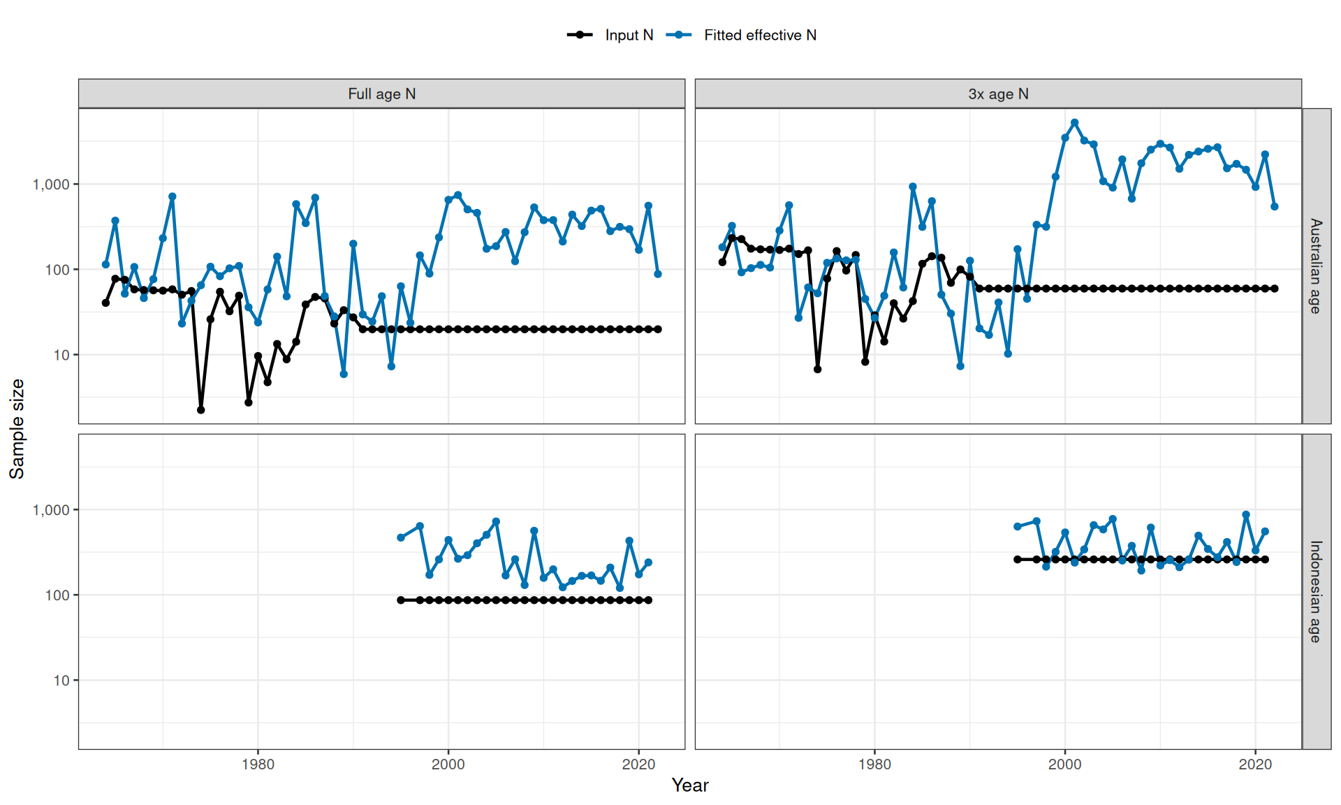
sample-size comparison in @tbl-triple-age-n-effn and @fig-triple-age-n-effn
provide additional checks on the 3x sensitivity.
```{r}
#| label: fit-standard-triple-age-n
#| echo: true
#| message: false
#| warning: false
summarise_standard_age_n_fit <- function(object, model_label) {
  rep <- object$report(object$env$last.par.best)
  tibble(
    model = model_label,
    convergence = object$opt$convergence,
    objective = object$fn(object$env$last.par.best),
    age_nll = sum(rep$lp_af),
    max_gradient = max(abs(object$gr(object$env$last.par.best)))
  )
}

mean_age_ci <- function(p, ages, N, level = 0.95) {
  p <- p / sum(p)
  mu <- sum(p * ages)
  var_mu <- (sum(p * ages^2) - mu^2) / N
  se <- sqrt(var_mu)
  z <- qnorm(1 - (1 - level) / 2)

  c(
    mean = mu,
    lower = mu - z * se,
    upper = mu + z * se,
    se = se
  )
}

make_age_mean_comparison <- function(data, object, sample_size_label) {
  rep <- object$report(object$env$last.par.best)
  fleet_names <- c(`5` = "Indonesian age", `6` = "Australian age")
  bind_rows(lapply(c(5, 6), function(f) {
    keep <- data$af_fishery == f & data$af_n > 0
    ages <- seq.int(unique(data$af_min_age[keep]), unique(data$af_max_age[keep]))
    cols <- ages + 1
    obs <- normalise_composition(data$af_obs[keep, cols, drop = FALSE])
    pred <- normalise_composition(rep$af_pred[keep, cols, drop = FALSE])
    obs_ci <- t(vapply(
      seq_len(nrow(obs)),
      function(i) mean_age_ci(obs[i, ], ages, data$af_n[keep][i]),
      numeric(4)
    ))
    tibble(
      sample_size = factor(
        sample_size_label,
        levels = c("Full age N", "3x age N")
      ),
      fishery = factor(
        fleet_names[as.character(f)],
        levels = c("Australian age", "Indonesian age")
      ),
      year = data$af_year[keep] + data$first_yr - 1,
      input_n = data$af_n[keep],
      observed = obs_ci[, "mean"],
      lower = obs_ci[, "lower"],
      upper = obs_ci[, "upper"],
      se = obs_ci[, "se"],
      predicted = as.vector(pred %*% ages)
    )
  }))
}

harmonic_mean <- function(x) {
  x <- x[!is.na(x) & x > 0]
  if (length(x) == 0) return(NA_real_)
  length(x) / sum(1 / x)
}

make_age_effective_n <- function(data, object, sample_size_label) {
  rep <- object$report(object$env$last.par.best)
  fleet_names <- c(`5` = "Indonesian age", `6` = "Australian age")
  bind_rows(lapply(c(5, 6), function(f) {
    keep <- data$af_fishery == f & data$af_n > 0
    ages <- seq.int(unique(data$af_min_age[keep]), unique(data$af_max_age[keep]))
    cols <- ages + 1
    obs <- normalise_composition(data$af_obs[keep, cols, drop = FALSE])
    pred <- normalise_composition(rep$af_pred[keep, cols, drop = FALSE])
    denominator <- rowSums((obs - pred)^2)
    numerator <- rowSums(pred * (1 - pred))
    tibble(
      sample_size = factor(
        sample_size_label,
        levels = c("Full age N", "3x age N")
      ),
      fishery = factor(
        fleet_names[as.character(f)],
        levels = c("Australian age", "Indonesian age")
      ),
      year = data$af_year[keep] + data$first_yr - 1,
      input_n = data$af_n[keep],
      eff_n = if_else(denominator > 0, numerator / denominator, Inf)
    )
  }))
}

make_osa_sample_size_by_model <- function(input) {
  sample_size <- collect_osa_sample_size(input) |>
    distinct(.data$model, .data$fleet, .data$index_label, .data$year, .data$N)

  ggplot(sample_size, aes(x = .data$year, y = .data$N)) +
    geom_col(fill = "#4C78A8", color = "#2F4F6F", width = 0.85, linewidth = 0.2) +
    facet_grid(.data$fleet ~ .data$model) +
    scale_y_continuous(labels = scales::label_comma()) +
    labs(x = "Year", y = "Input sample size (N)") +
    theme_bw(base_size = 10)
}

triple_age_n_data <- default_fit$data
triple_age_n_rows <- triple_age_n_data$af_fishery %in% c(5, 6) &
  triple_age_n_data$af_n > 0
triple_age_n_data$af_n[triple_age_n_rows] <- triple_age_n_data$af_n[triple_age_n_rows] * 3

triple_age_n_parameters <- update_parameters_from_fit(default_fit$parameters, default_obj)
triple_age_n_obj <- MakeADFun(
  func = cmb(sbt_model, triple_age_n_data),
  parameters = triple_age_n_parameters,
  map = default_fit$map,
  silent = TRUE
)
triple_age_n_bounds <- get_bounds(
  triple_age_n_obj,
  parameters = triple_age_n_parameters
)
triple_age_n_opt <- run_or_load_nlminb(
  cache_name = "standard_selectivity_triple_age_n",
  object = triple_age_n_obj,
  bounds = triple_age_n_bounds,
  control = control,
  n_passes = 3
)
triple_age_n_obj$par <- triple_age_n_opt$par
triple_age_n_obj$env$last.par.best <- triple_age_n_opt$par
triple_age_n_obj$fn(triple_age_n_opt$par)
triple_age_n_obj$opt <- triple_age_n_opt

triple_age_n_fit_summary <- bind_rows(
  summarise_standard_age_n_fit(default_obj, "Standard selectivity"),
  summarise_standard_age_n_fit(triple_age_n_obj, "Standard (3x age N)")
)

triple_age_n_osa_age <- c(
  make_age_osa(default_fit$data, default_obj, "Standard selectivity"),
  make_age_osa(triple_age_n_data, triple_age_n_obj, "Standard (3x age N)")
)

triple_age_n_mean_age <- bind_rows(
  make_age_mean_comparison(default_fit$data, default_obj, "Full age N"),
  make_age_mean_comparison(triple_age_n_data, triple_age_n_obj, "3x age N")
)

triple_age_n_mean_age_plot <- ggplot(triple_age_n_mean_age, aes(x = .data$year)) +
  geom_errorbar(
    aes(ymin = .data$lower, ymax = .data$upper, color = "Observed 95% CI"),
    width = 0,
    linewidth = 0.45
  ) +
  geom_point(aes(y = .data$observed, color = "Observed mean"), size = 1.5) +
  geom_line(aes(y = .data$predicted, color = "Predicted mean"), linewidth = 0.8) +
  facet_grid(.data$fishery ~ .data$sample_size, scales = "free_y") +
  scale_color_manual(
    values = c(
      "Observed mean" = "black",
      "Observed 95% CI" = "grey45",
      "Predicted mean" = "#D55E00"
    )
  ) +
  labs(x = "Year", y = "Mean age", color = NULL) +
  theme_bw(base_size = 10) +
  theme(legend.position = "top")

triple_age_n_eff_n <- bind_rows(
  make_age_effective_n(default_fit$data, default_obj, "Full age N"),
  make_age_effective_n(triple_age_n_data, triple_age_n_obj, "3x age N")
)

triple_age_n_eff_n_summary <- triple_age_n_eff_n |>
  group_by(.data$sample_size, .data$fishery) |>
  summarise(
    n_years = n(),
    mean_input_n = mean(.data$input_n),
    harmonic_eff_n = harmonic_mean(.data$eff_n),
    median_eff_n = median(.data$eff_n),
    .groups = "drop"
  ) |>
  mutate(
    harmonic_eff_n_over_mean_input_n = .data$harmonic_eff_n / .data$mean_input_n
  )

triple_age_n_eff_n_plot_data <- triple_age_n_eff_n |>
  pivot_longer(
    cols = c("input_n", "eff_n"),
    names_to = "series",
    values_to = "N"
  ) |>
  mutate(
    series = recode(
      .data$series,
      input_n = "Input N",
      eff_n = "Fitted effective N"
    ),
    series = factor(.data$series, levels = c("Input N", "Fitted effective N"))
  ) |>
  filter(is.finite(.data$N), .data$N > 0)

triple_age_n_eff_n_plot <- ggplot(
  triple_age_n_eff_n_plot_data,
  aes(x = .data$year, y = .data$N, color = .data$series)
) +
  geom_line(linewidth = 0.8) +
  geom_point(size = 1.4) +
  facet_grid(.data$fishery ~ .data$sample_size) +
  scale_y_log10(labels = scales::label_comma()) +
  scale_color_manual(values = c("Input N" = "black", "Fitted effective N" = "#0072B2")) +
  labs(x = "Year", y = "Sample size", color = NULL) +
  theme_bw(base_size = 10) +
  theme(legend.position = "top")

triple_age_n_osa_plot_parts <- list(
  n = make_osa_sample_size_by_model(triple_age_n_osa_age),
  pearson = make_osa_pearson_bubble(triple_age_n_osa_age),
  qq = make_osa_qq(triple_age_n_osa_age),
  aggcomp = make_osa_agg(triple_age_n_osa_age)
)

triple_age_n_osa_sdnr <- summarise_osa_sdnr(
  triple_age_n_osa_age,
  "Age composition"
)

triple_age_n_selectivity_indo <- bind_rows(
  collect_selectivity(default_fit$data, default_obj, "Standard selectivity", "Indonesian"),
  collect_selectivity(triple_age_n_data, triple_age_n_obj, "Standard (3x age N)", "Indonesian")
)

triple_age_n_selectivity_ranges_indo <- bind_rows(
  collect_selectivity_ranges(default_fit$data, "Standard selectivity", "Indonesian"),
  collect_selectivity_ranges(triple_age_n_data, "Standard (3x age N)", "Indonesian")
)

triple_age_n_selectivity_indo_plot <- plot_selectivity_data(
  triple_age_n_selectivity_indo,
  triple_age_n_selectivity_ranges_indo,
  years = data$first_yr_catch_f[5]:data$last_yr
)
```
```{r}
#| label: tbl-triple-age-n-fit
#| echo: false
#| tbl-cap: "Standard selectivity fit summary after tripling Indonesian and Australian age-composition sample sizes."
triple_age_n_fit_summary |>
mutate(
objective = round(.data$objective, 3),
age_nll = round(.data$age_nll, 3),
max_gradient = formatC(
.data$max_gradient,
format = "e",
digits = 2
)
) |>
knitr::kable()
```
```{r}
#| label: tbl-triple-age-n-osa-sdnr
#| echo: false
#| tbl-cap: "Age-composition OSA SDNR diagnostics for the standard model and the 3x age-composition sample-size refit."
triple_age_n_osa_sdnr |>
arrange(.data$fleet, .data$model) |>
knitr::kable()
```
Tripling the age-composition sample sizes increases the weight assigned to the
Indonesian and Australian age compositions in the standard selectivity fit.
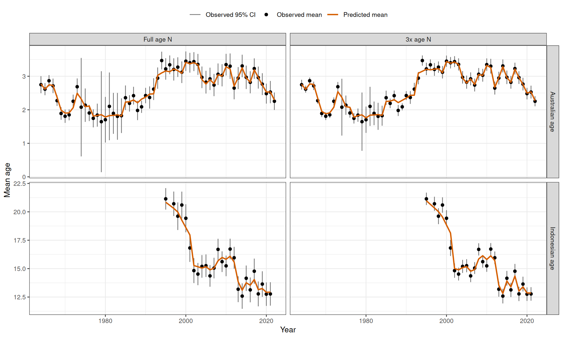
The observed mean-age confidence intervals in @fig-triple-age-n-mean-age use
the tripled input sample sizes in the 3x facet, so the intervals narrow
relative to the full-`N` comparison. The predicted mean-age lines show how the
standard selectivity fit changes when the age compositions are forced to carry
more influence in the objective function.
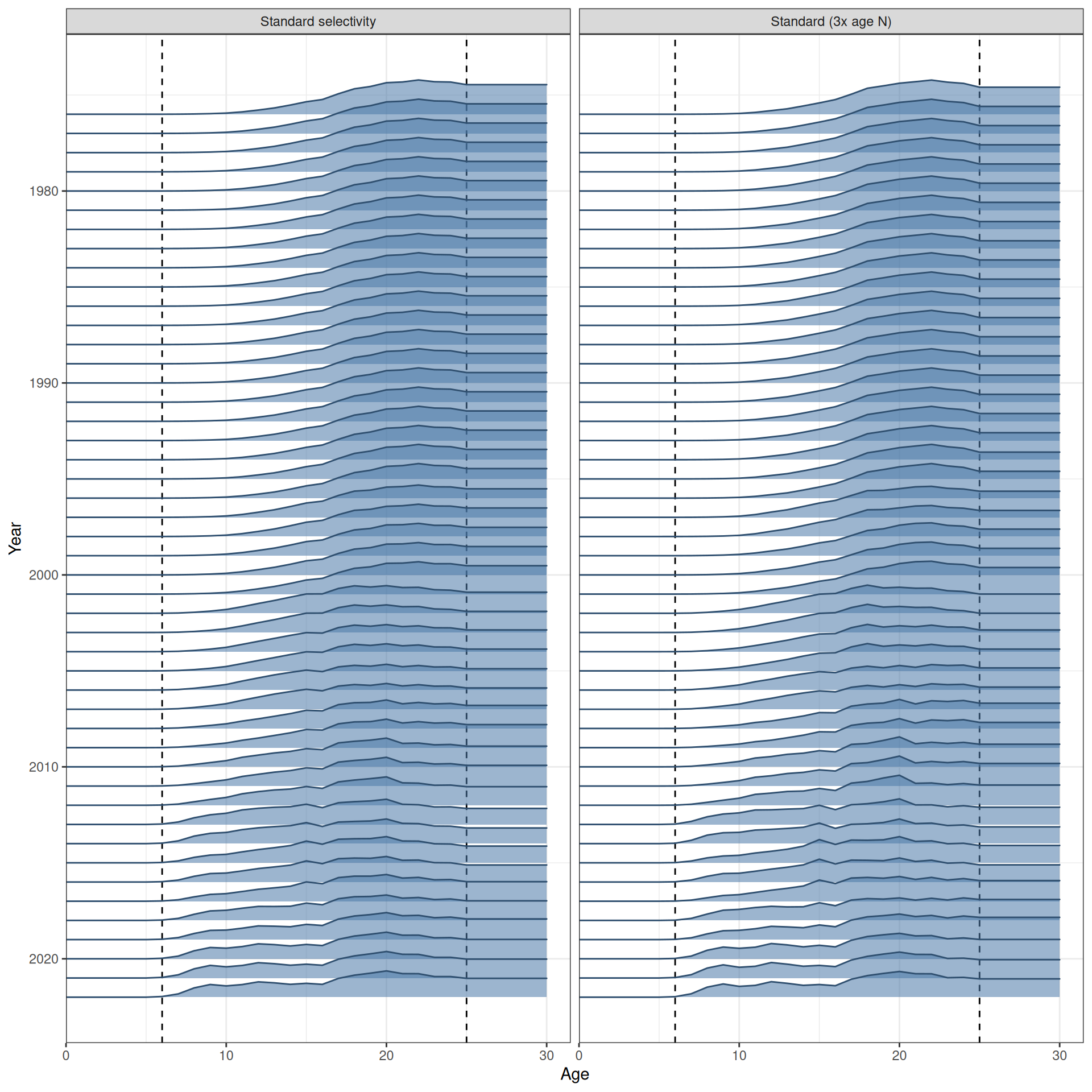
The Indonesian selectivity estimates in @fig-triple-age-n-selectivity-indo
show whether the increased age-composition weighting changes the standard
selectivity surface for the fishery that carries the older age-composition
signal.
```{r}
#| label: fig-triple-age-n-mean-age
#| echo: true
#| message: false
#| warning: false
#| fig-width: 10
#| fig-height: 6
#| fig-cap: Observed mean age with input-sample-size-based 95% confidence intervals and predicted mean age lines for the Indonesian and Australian age-composition fisheries under the original and 3x age-composition sample-size standard selectivity fits.
triple_age_n_mean_age_plot
```
```{r}
#| label: fig-triple-age-n-selectivity-indo
#| echo: true
#| message: false
#| warning: false
#| fig-width: 10
#| fig-height: 10
#| fig-cap: Side-by-side comparison of fitted Indonesian selectivity at age by year under the original and 3x age-composition sample-size standard selectivity fits.
triple_age_n_selectivity_indo_plot
```
```{r}
#| label: tbl-triple-age-n-effn
#| echo: false
#| tbl-cap: "McAllister-Ianelli effective sample-size summaries for the 3x Indonesian and Australian age-composition sample-size sensitivity."
triple_age_n_eff_n_summary |>
mutate(
mean_input_n = round(.data$mean_input_n, 1),
harmonic_eff_n = round(.data$harmonic_eff_n, 1),
median_eff_n = round(.data$median_eff_n, 1),
harmonic_eff_n_over_mean_input_n = round(.data$harmonic_eff_n_over_mean_input_n, 3)
) |>
knitr::kable()
```
```{r}
#| label: fig-triple-age-n-effn
#| echo: true
#| message: false
#| warning: false
#| fig-width: 10
#| fig-height: 6
#| fig-cap: Input sample size and fitted McAllister-Ianelli effective sample size by year for the Indonesian and Australian age-composition fisheries under the original and 3x age-composition sample-size standard selectivity fits.
triple_age_n_eff_n_plot
```
```{r}
#| label: fig-triple-age-n-osa-age-n
#| echo: true
#| message: false
#| warning: false
#| fig-width: 10
#| fig-height: 6
#| fig-cap: Input sample sizes used for age-composition OSA diagnostics under the original and 3x age-composition sample-size standard selectivity fits.
triple_age_n_osa_plot_parts$n
```
```{r}
#| label: fig-triple-age-n-osa-age-pearson
#| echo: true
#| message: false
#| warning: false
#| fig-width: 10
#| fig-height: 6
#| fig-cap: Pearson residual bubble plots for age compositions under the original and 3x age-composition sample-size standard selectivity fits.
triple_age_n_osa_plot_parts$pearson
```
```{r}
#| label: fig-triple-age-n-osa-age-qq
#| echo: true
#| message: false
#| warning: false
#| fig-width: 10
#| fig-height: 6
#| fig-cap: OSA Q-Q plots for age compositions under the original and 3x age-composition sample-size standard selectivity fits.
triple_age_n_osa_plot_parts$qq
```
```{r}
#| label: fig-triple-age-n-osa-age-agg
#| echo: true
#| message: false
#| warning: false
#| fig-width: 10
#| fig-height: 6
#| fig-cap: Aggregate OSA fits for age compositions under the original and 3x age-composition sample-size standard selectivity fits.
triple_age_n_osa_plot_parts$aggcomp
```
# References