| ADMB | RTMB | Difference | Percent difference | |
|---|---|---|---|---|
| Parameters | ||||
| B0 | 1.08358e+07 | 1.083578e+07 | 18.0862526 | 0.0002 |
| psi | 1.50000e+00 | 1.500000e+00 | 0.0000000 | 0.0000 |
| sigmaR | 6.00000e-01 | 6.000000e-01 | 0.0000000 | 0.0000 |
| h | 5.50000e-01 | 5.500000e-01 | 0.0000000 | 0.0000 |
| q HSP | 1.00000e+00 | 1.000000e+00 | 0.0000000 | 0.0000 |
| m0 | 4.00000e-01 | 4.000000e-01 | 0.0000000 | 0.0000 |
| m4 | 1.67050e-01 | 1.670507e-01 | -0.0000007 | 0.0004 |
| m10 | 6.50000e-02 | 6.500000e-02 | 0.0000000 | 0.0000 |
| m30 | 4.57410e-01 | 4.574100e-01 | 0.0000000 | 0.0000 |
| Derived quantities | ||||
| R0 | 8.74439e+06 | 8.744386e+06 | 3.9612256 | 0.0000 |
| alpha | 1.09929e+07 | 1.099294e+07 | -42.4487450 | 0.0004 |
| beta | 2.78634e+06 | 2.786344e+06 | -3.9206779 | 0.0001 |
| tau_ac2 | 6.44716e-01 | 6.447156e-01 | 0.0000004 | 0.0001 |
| Priors & penalties | ||||
| kludge | 0.00000e+00 | 0.000000e+00 | 0.0000000 | 0.0000 |
| sel.change | 7.06247e+01 | 7.062467e+01 | 0.0000305 | 0.0000 |
| sel.smooth | 3.42249e+01 | 3.422494e+01 | -0.0000408 | 0.0001 |
| rec | -3.03390e+01 | -3.033900e+01 | 0.0000045 | 0.0000 |
| m0 | 0.00000e+00 | 0.000000e+00 | 0.0000000 | 0.0000 |
| m10 | 0.00000e+00 | 0.000000e+00 | 0.0000000 | 0.0000 |
| steep | 0.00000e+00 | 0.000000e+00 | 0.0000000 | 0.0000 |
| omega | 0.00000e+00 | 0.000000e+00 | 0.0000000 | 0.0000 |
| expl | 0.00000e+00 | 0.000000e+00 | 0.0000000 | 0.0000 |
| sel.init | 2.00000e-07 | 2.000000e-07 | 0.0000000 | 0.0002 |
| hstar | 7.63360e+00 | 7.633597e+00 | 0.0000030 | 0.0000 |
| Likelihoods & objective function | ||||
| LL1 | 1.94607e+02 | 1.946072e+02 | -0.0002198 | 0.0001 |
| LL2 | 3.09202e+01 | 3.092031e+01 | -0.0001054 | 0.0003 |
| LL3 | 3.48981e+01 | 3.489813e+01 | -0.0000286 | 0.0001 |
| LL4 | 3.82627e+01 | 3.826276e+01 | -0.0000591 | 0.0002 |
| Indo | 9.30514e+01 | 9.305138e+01 | 0.0000202 | 0.0000 |
| Aus | 4.54265e+01 | 4.542650e+01 | -0.0000019 | 0.0000 |
| CPUE | -6.46131e+01 | -6.461295e+01 | -0.0001494 | 0.0002 |
| Tags | 1.76553e+02 | 1.765530e+02 | 0.0000081 | 0.0000 |
| Aerial | 3.98139e+00 | 3.981441e+00 | -0.0000505 | 0.0013 |
| Troll | -1.20015e+01 | -1.200157e+01 | 0.0000656 | 0.0005 |
| POP | 1.75465e+03 | 1.754654e+03 | -0.0037102 | 0.0002 |
| HSP | 2.19884e+03 | 2.199118e+03 | -0.2776306 | 0.0126 |
| GT | 1.45904e+03 | 1.459035e+03 | 0.0046028 | 0.0003 |
| ObjF | 6.03576e+03 | 6.036037e+03 | -0.2771518 | 0.0046 |
Introduction
This vignette compares outputs from the ADMB model to the RTMB model within the sbt package. This is done using a fixed parameter run and then by optimising. In the fixed parameter run the parameter values from a single cell of the ADMB model are used as fixed value inputs to sbt and outputs from sbt are generated then compared to the ADMB outputs.
Fixed parameter run
Comparison table
Table 1 includes transformed parameters (i.e., in natural space), derived quantities, priors, penalties, likelihoods, and objective function values for the ADMB model, the RTMB model, and the difference and percent difference between the two models:
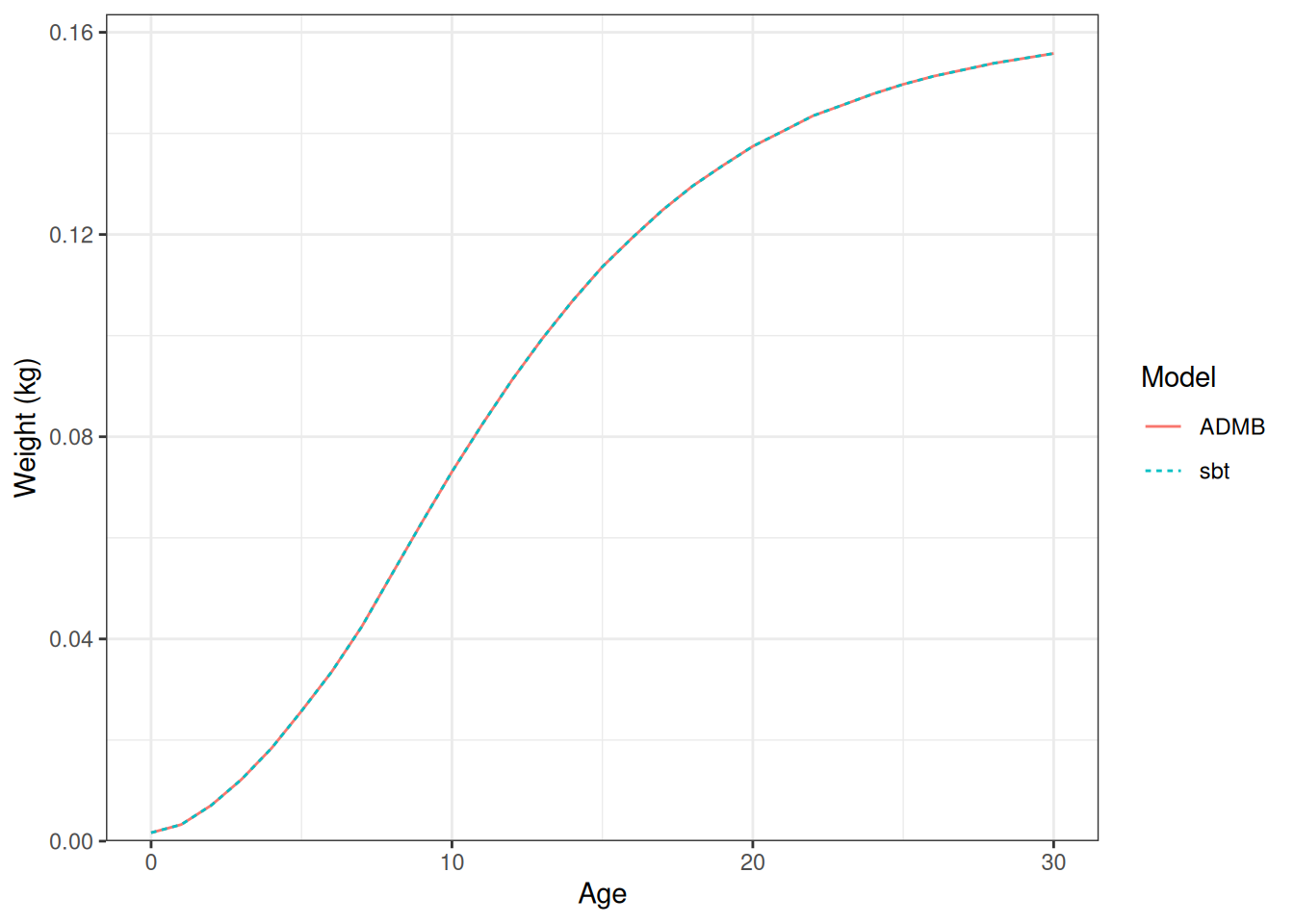
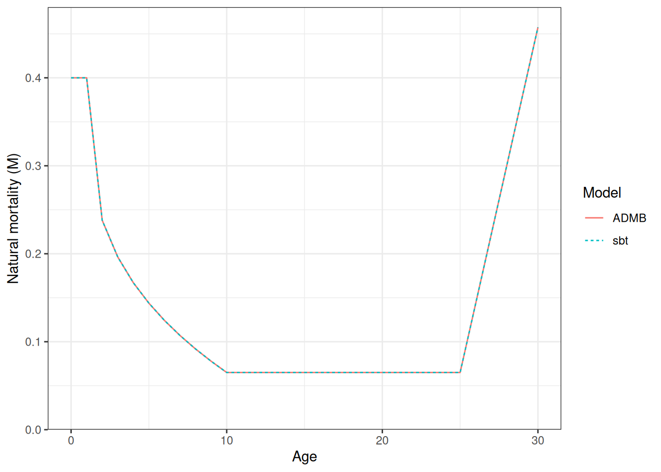
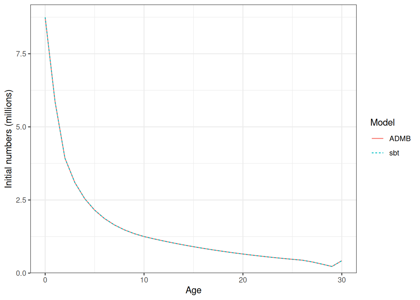
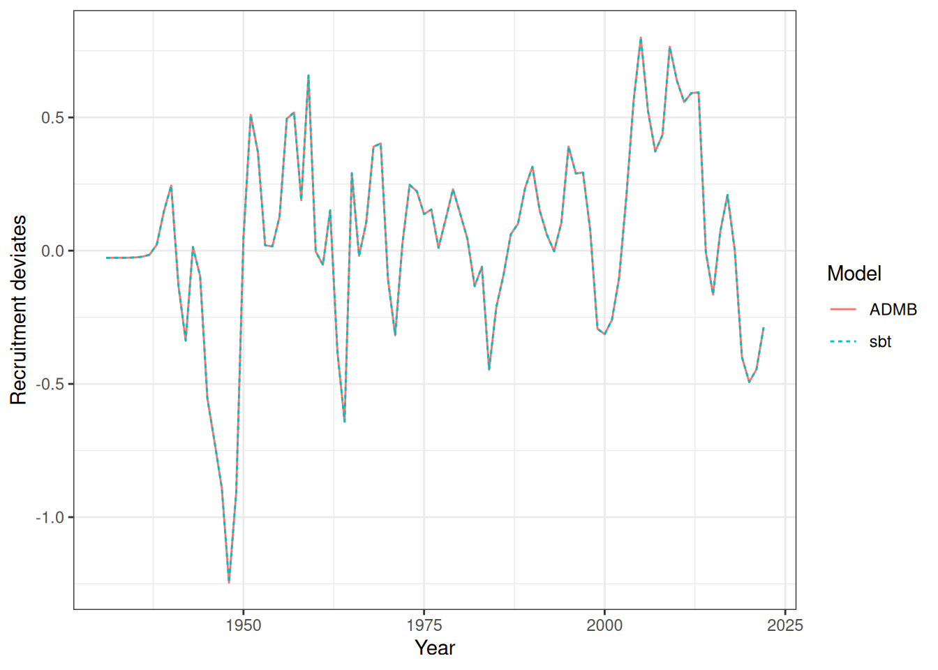
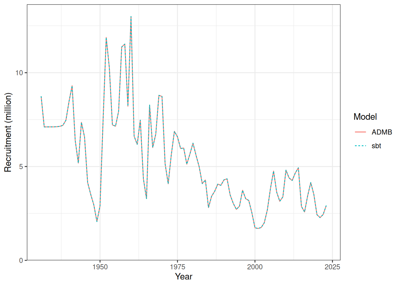
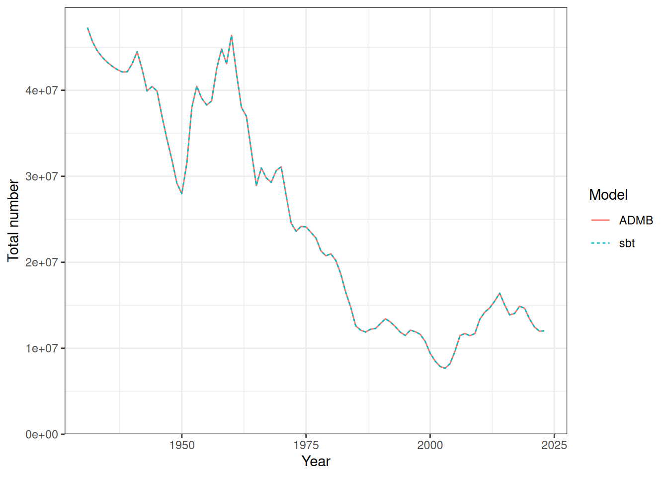
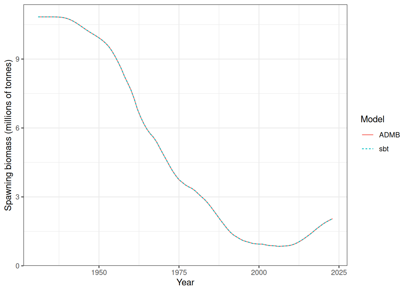
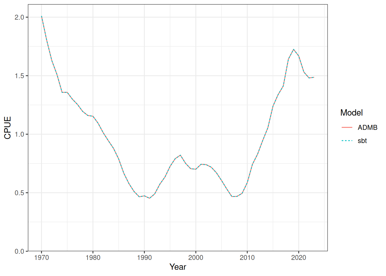
Comparison figures
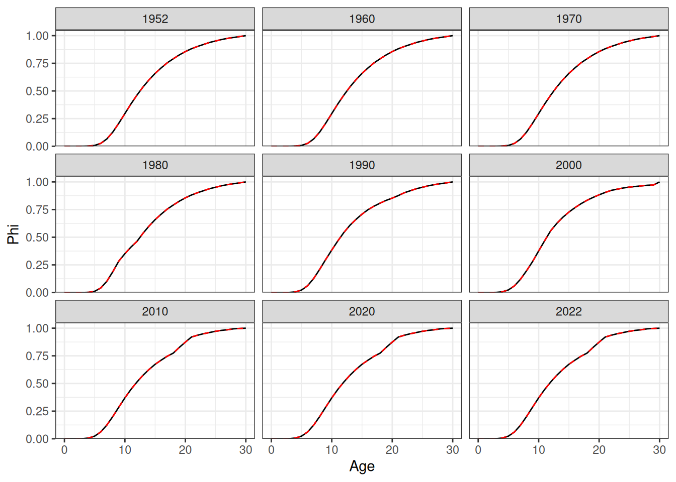
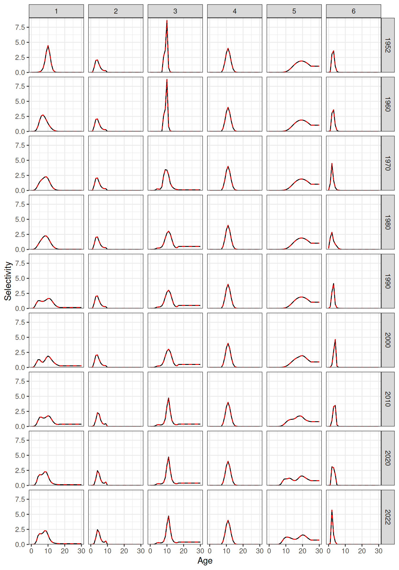
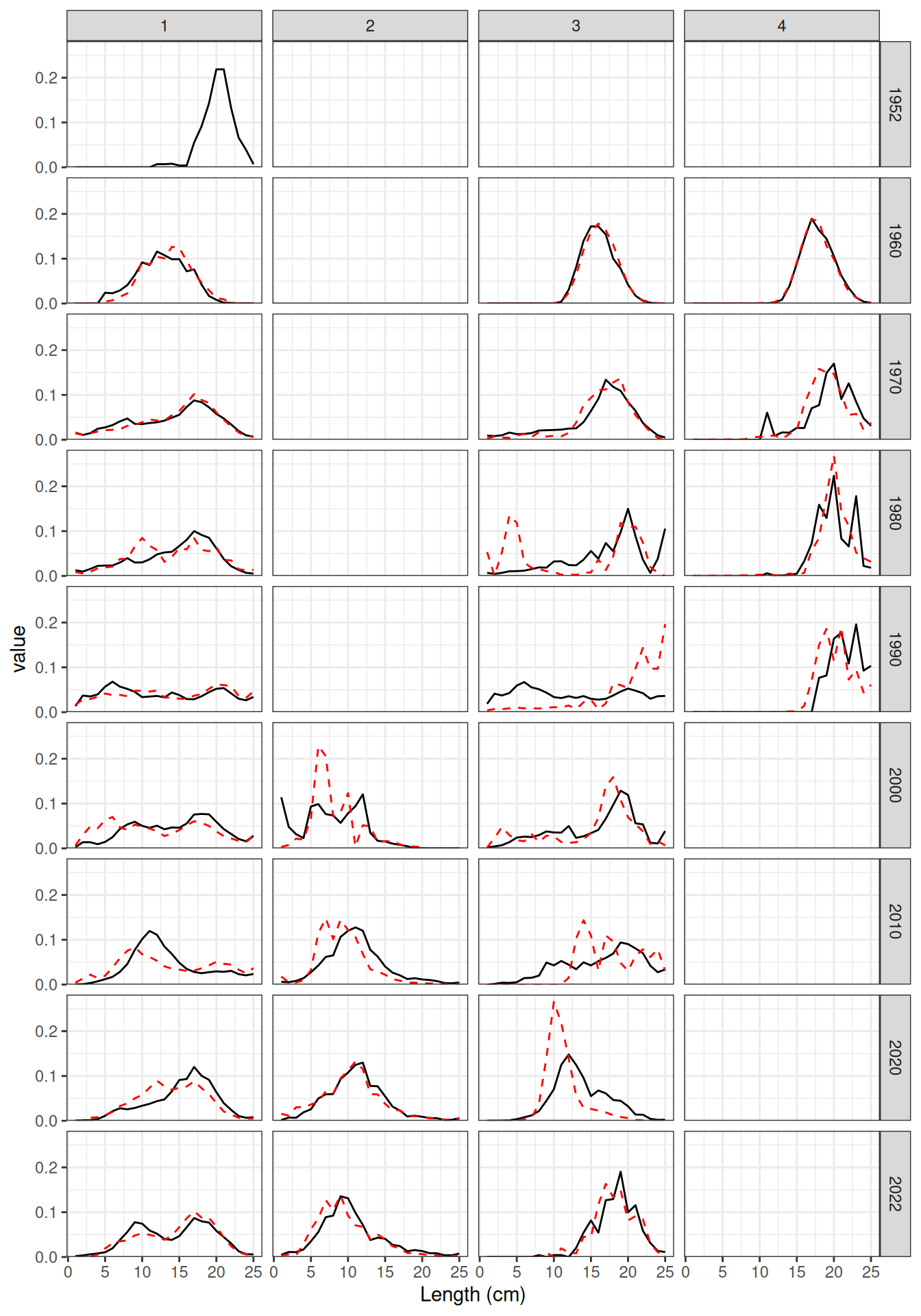
The following figures compare outputs from the ADMB and RTMB models: average weight at age (Figure 1), natural mortality at age (Figure 2), initial numbers at age (Figure 3), recruitment deviates (Figure 4), recruitment (Figure 5), total numbers (Figure 6), spawning biomass (Figure 7), CPUE (Figure 8), phi at age (Figure 9), selectivity at age (Figure 10), and age-frequency observations and predictions (Figure 12, Figure 13).
There was a reason why the LF observations are different (Figure 11) but I cannot remember why. Must be something to do with post processing in the code as the likelihoods are the same.
#> [1] NA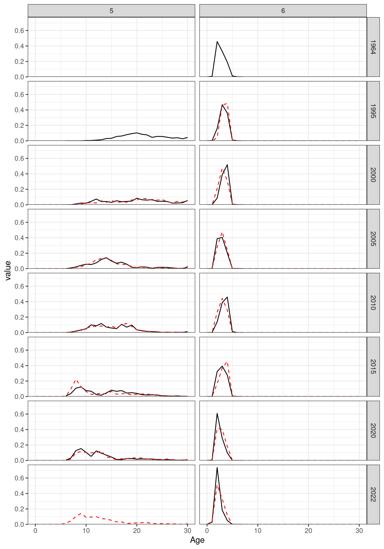
#> [1] NA NA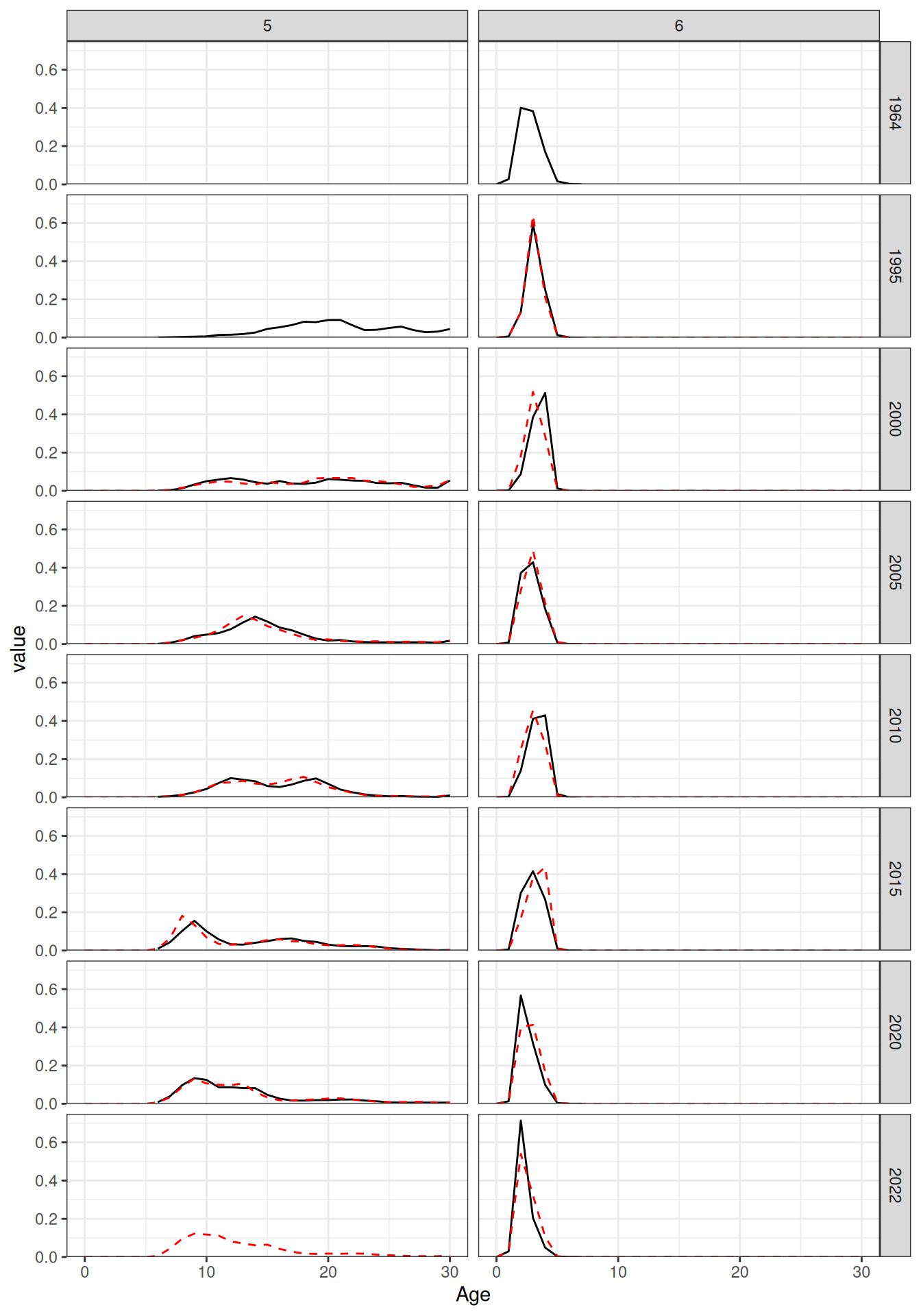
Optimising
Now the model is optimised using nlminb to see if RTMB produces the same result. The nlminb function finds the same optimum as ADMB (Figure 14):
