Introduction
The sbt software is an R package (R Core Team 2024) that contains the CCSBT operating model (OM) coded using RTMB Kristensen (2025). This page provides examples using the sbt model.
Load inputs
If you have not done so already, you will need to install the following R packages:
remotes::install_github("janoleko/RTMBdist")
remotes::install_github("andrjohns/StanEstimators")
remotes::install_github("noaa-afsc/SparseNUTS")
The sbt RTMB model is loaded along with several R functions using library(sbt). The tidyverse and reshape2 packages are used for data manipulation and plotting. The code theme_set(theme_bw()) alters the plot aesthetics of the entire article:
Model setup
Define the parameter list:
parameters <- get_parameters(data = data)
names(parameters)
[1] "par_log_B0" "par_log_psi" "par_log_m0"
[4] "par_log_m4" "par_log_m10" "par_log_m30"
[7] "par_log_h" "par_log_sigma_r" "par_log_cpue_q"
[10] "par_cpue_creep" "par_log_cpue_sigma" "par_log_cpue_omega"
[13] "par_log_aerial_tau" "par_log_aerial_sel" "par_log_troll_tau"
[16] "par_log_gt_q" "par_log_hsp_q" "par_log_tag_H_factor"
[19] "par_log_af_alpha" "par_log_lf_alpha" "par_sel_rho_y"
[22] "par_sel_rho_a" "par_log_sel_sigma" "par_log_sel_1"
[25] "par_log_sel_2" "par_log_sel_3" "par_log_sel_4"
[28] "par_log_sel_5" "par_log_sel_6" "par_log_sel_7"
[31] "par_rdev_y" There is a lot of flexibility in specifying priors now. The default priors are loaded using get_priors and the evaluate_priors function can be used to check that the priors are doing what you expect:
data$priors <- get_priors(parameters = parameters)
evaluate_priors(parameters = parameters, priors = data$priors)
[1] 61.73913Use RTMB’s map option to turn parameters on/off:
map <- get_map(parameters = parameters)Using the data, the parameters, the parameter map, and the model (sbt_model), the AD object is created using RTMBs MakeADFun function:
obj <- MakeADFun(func = cmb(sbt_model, data), parameters = parameters, map = map)The parameters that are being estimated can be viewed using:
 [1] "par_log_B0"     "par_log_m4"     "par_log_m30"    "par_log_cpue_q"
 [5] "par_log_sel_1"  "par_log_sel_2"  "par_log_sel_3"  "par_log_sel_5"
 [9] "par_log_sel_6"  "par_log_sel_7"  "par_rdev_y"
The objective function value given the initial parameter values is:
obj$fn(obj$par)[1] 25861.77Load the default parameter bounds:
bounds <- get_bounds(obj, parameters = parameters)Optimisation
Optimisation of the model parameters is done using the nlminb function:
control <- list(eval.max = 10000, iter.max = 10000)
opt <- nlminb(start = obj$par,
              objective = obj$fn, gradient = obj$gr, hessian = obj$he,
              control = control, lower = bounds$lower, upper = bounds$upper)
opt <- nlminb(start = opt$par,
              objective = obj$fn, gradient = obj$gr, hessian = obj$he,
              control = control, lower = bounds$lower, upper = bounds$upper)
Check that all parameters are estimable using the check_estimability function. This function was taken from the TMBhelper package and added to the sbt package because the TMBhelper package is not set up as a proper package (it does not install properly on the GitHub servers).
check_estimability(obj = obj)Model fits
Model fit to CPUE (Figure 1) and the aerial surveys (Figure 2). Length frequency fits for each longline fleet are shown in Figure 3, Figure 4, Figure 5, and Figure 6. Age composition fits are shown for the Indonesian fleet (Figure 7) and the Australian fleet (Figure 8).
plot_cpue(data = data, object = obj, nsim = 10)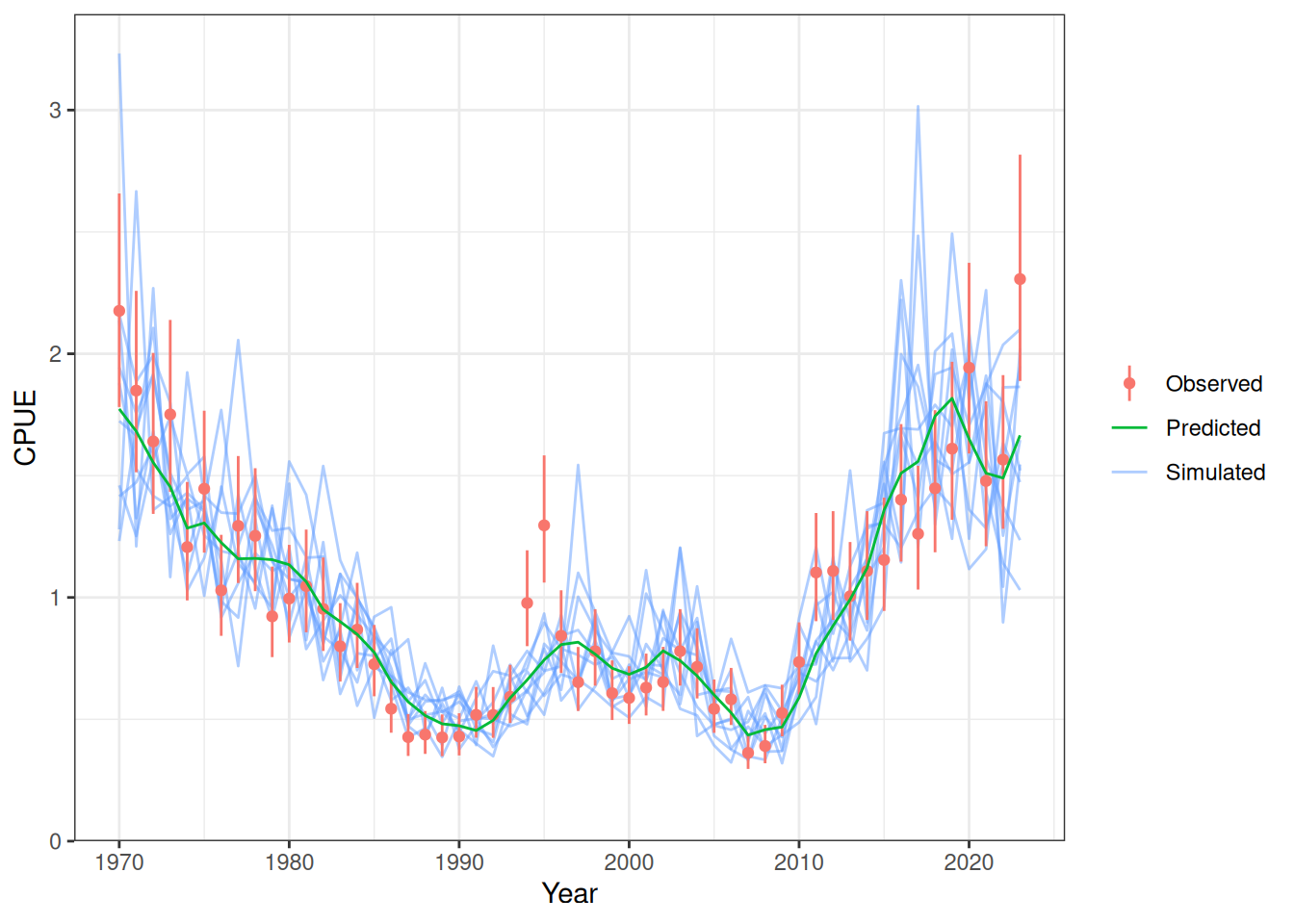
plot_aerial_survey(data = data, object = obj, nsim = 10)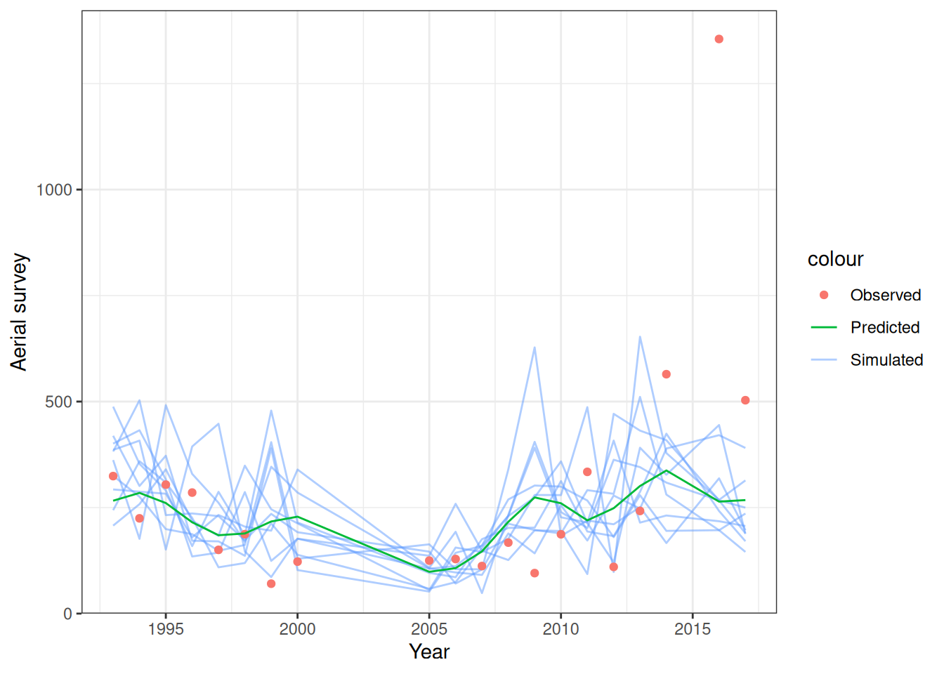
plot_lf(data = data, object = obj, fishery = "LL1", ncol = 5)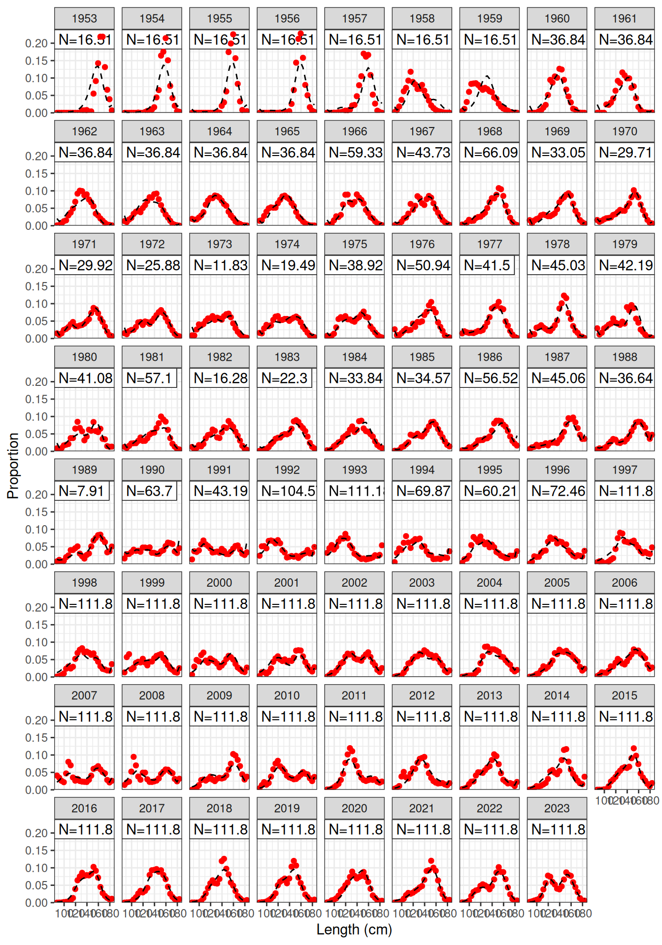
plot_lf(data = data, object = obj, fishery = "LL2", ncol = 5)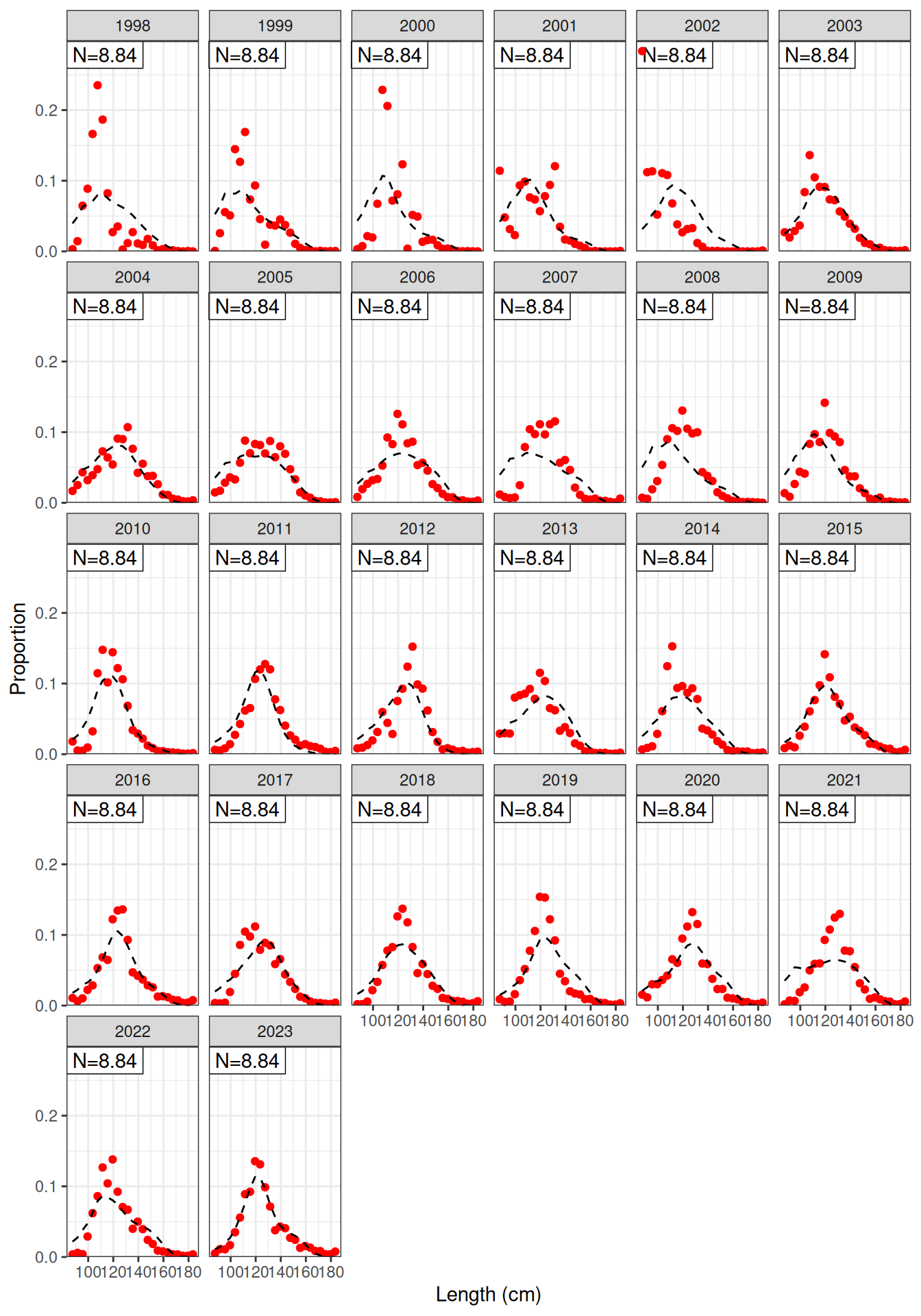
plot_lf(data = data, object = obj, fishery = "LL3", ncol = 5)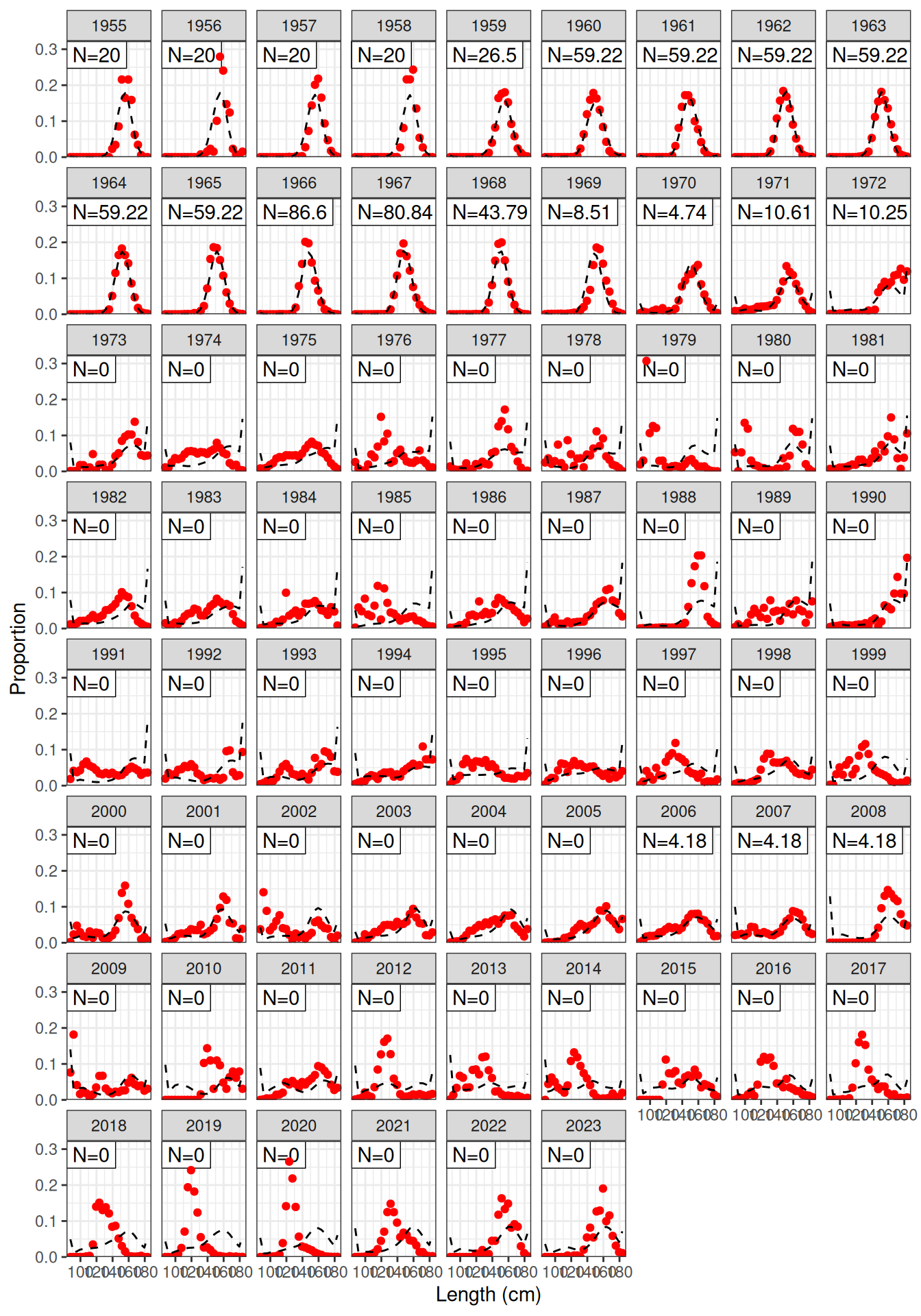
plot_lf(data = data, object = obj, fishery = "LL4", ncol = 5)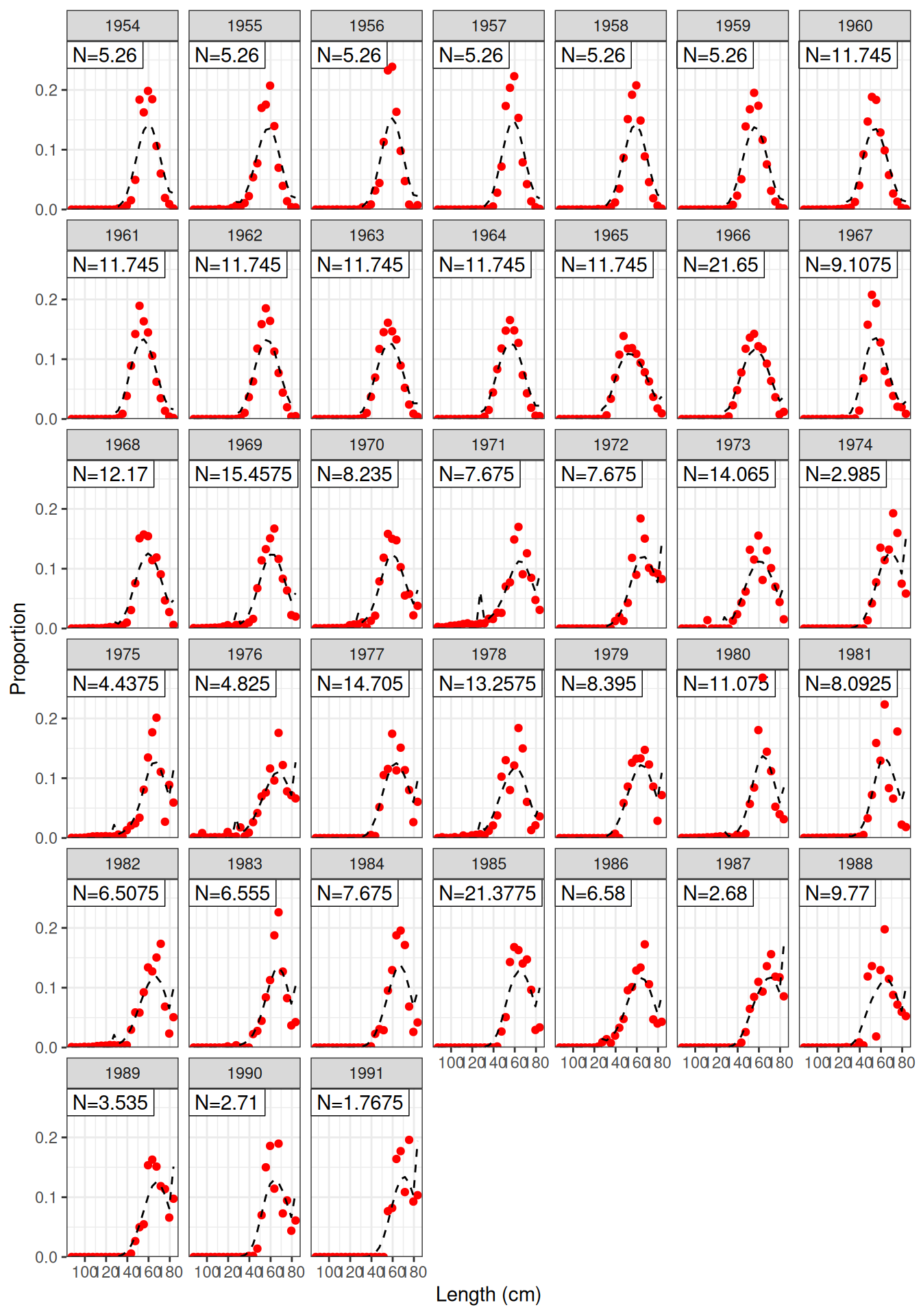
plot_af(data = data, object = obj, fishery = "Indonesian")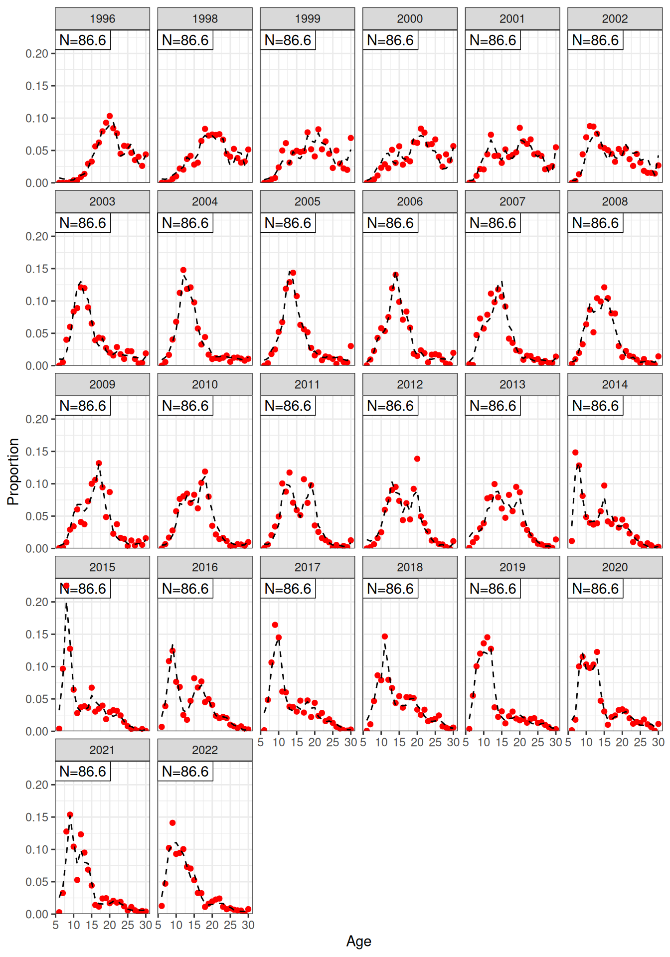
plot_af(data = data, object = obj, fishery = "Australian")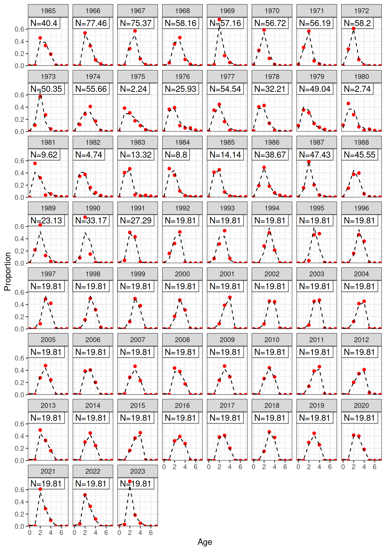
I think that not all of the catch is being taken for LL4 because there are years where there is catch but no LFs but we’ve set this fishery to direct removals (Figure 9, Figure 10).
plot_catch(data = data, object = obj)[1] "The maximum catch difference was: 18.98"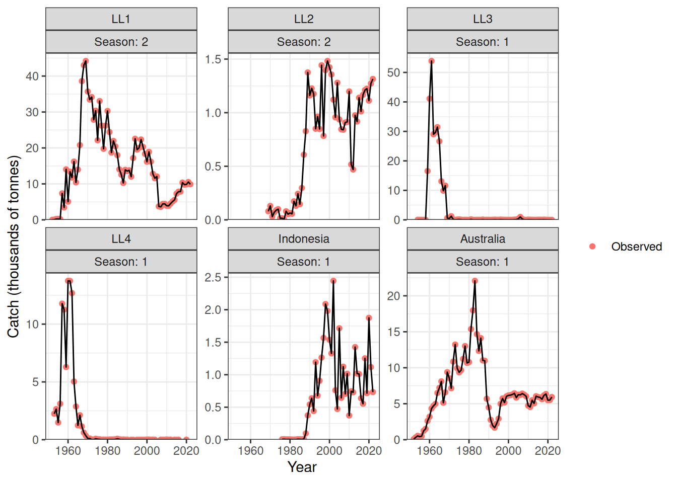
plot_catch(data = data, object = obj, plot_resid = TRUE)[1] "The maximum catch difference was: 18.98"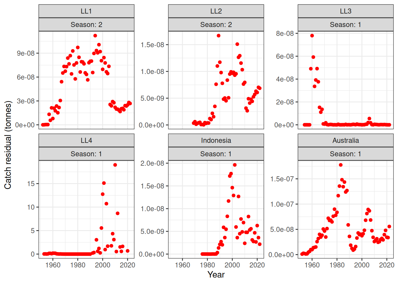
One step ahead (OSA) residuals
One step ahead (OSA) residuals are a replacement for Pearson residuals (Figure 11).
osa_cpue <- oneStepPredict(obj = obj, observation.name = "cpue_log_obs",
                           method = "oneStepGeneric", trace = FALSE)
qqnorm(osa_cpue$res); abline(0, 1)
# plot(osa_cpue$res); abline(-2, 0); abline(0, 0); abline(2, 0)
# osa <- oneStepPredict(obj = obj, method = "fullGaussian", discrete = FALSE, trace = FALSE)
# osa_troll <- oneStepPredict(obj = obj, observation.name = "troll_log_obs", method = "oneStepGeneric", trace = FALSE)
# qqnorm(osa_troll$res); abline(0, 1)
# plot(osa_troll$res); abline(0, 0)
# osa_aerial <- oneStepPredict(obj = obj, observation.name = "aerial_log_obs", method = "oneStepGeneric", trace = FALSE)
# qqnorm(osa$res); abline(0, 1)
# osa_gt <- oneStepPredict(obj = obj, observation.name = "gt_nrec", method = "oneStepGeneric", discrete = TRUE, trace = FALSE)
# qqnorm(osa_gt$res); abline(0, 1)
# plot(osa_gt$res); abline(-2, 0); abline(0, 0); abline(2, 0)
# osa_hsp <- oneStepPredict(obj = obj, observation.name = "hsp_nK", method = "oneStepGeneric", discrete = TRUE, trace = FALSE)
# qqnorm(osa_hsp$res); abline(0, 1)
# plot(osa_hsp$res); abline(0, 0)
# osa_pop <- oneStepPredict(obj = obj, observation.name = "pop_nP", method = "oneStepGeneric", discrete = TRUE, trace = FALSE)
# qqnorm(osa_pop$res); abline(0, 1)
# plot(osa_pop$res); abline(0, 0)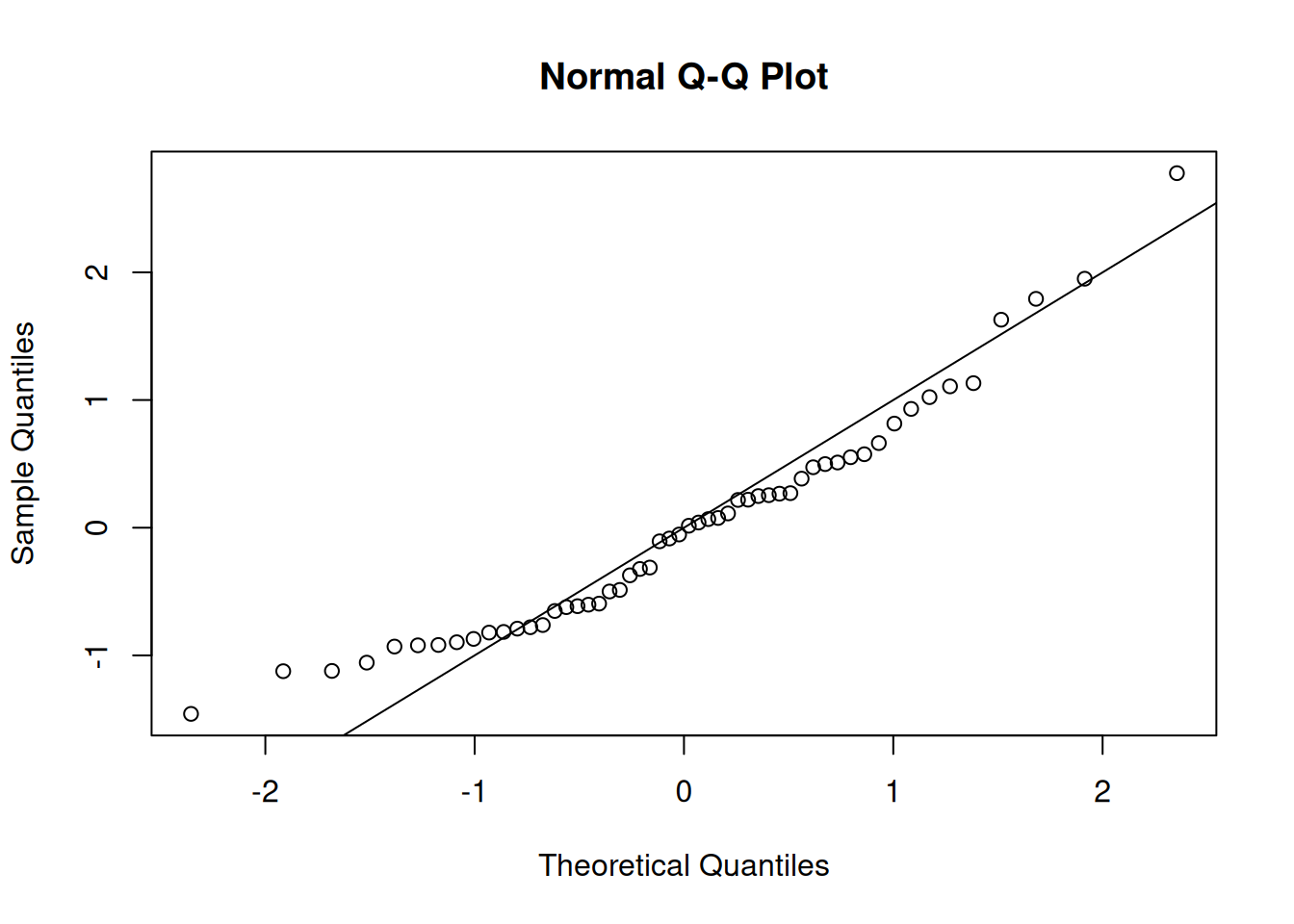
Derived quantities
Recruitment deviates and recruitment (Figure 12, Figure 13). Natural mortality at age is shown in Figure 14. Initial numbers at age are shown in Figure 15. Harvest rates are shown in Figure 16.
plot_rec_devs(data = data, object = obj)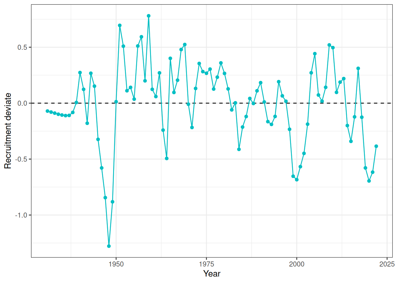
plot_recruitment(data = data, object = obj)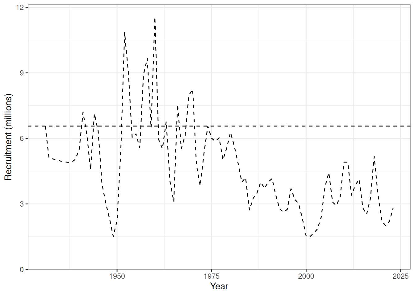
plot_natural_mortality(data = data, object = obj)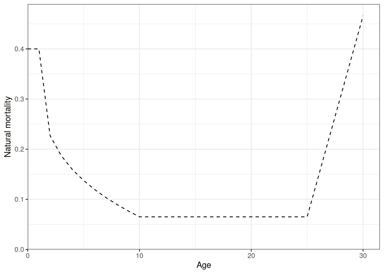
plot_initial_numbers(data = data, object = obj)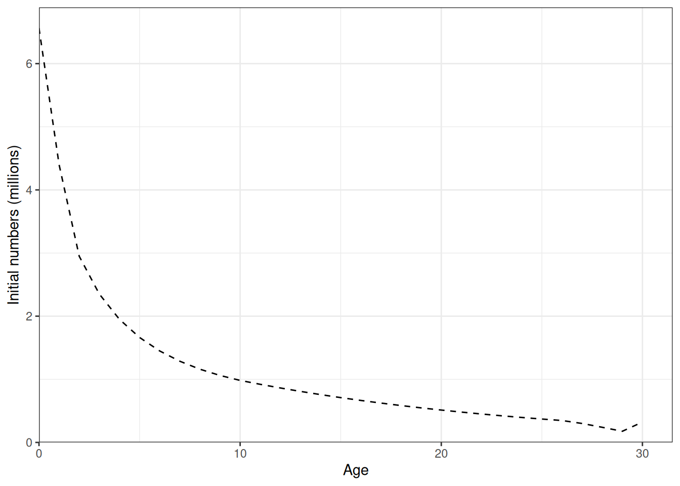
plot_hrate(data = data, object = obj, years = 1990:2010)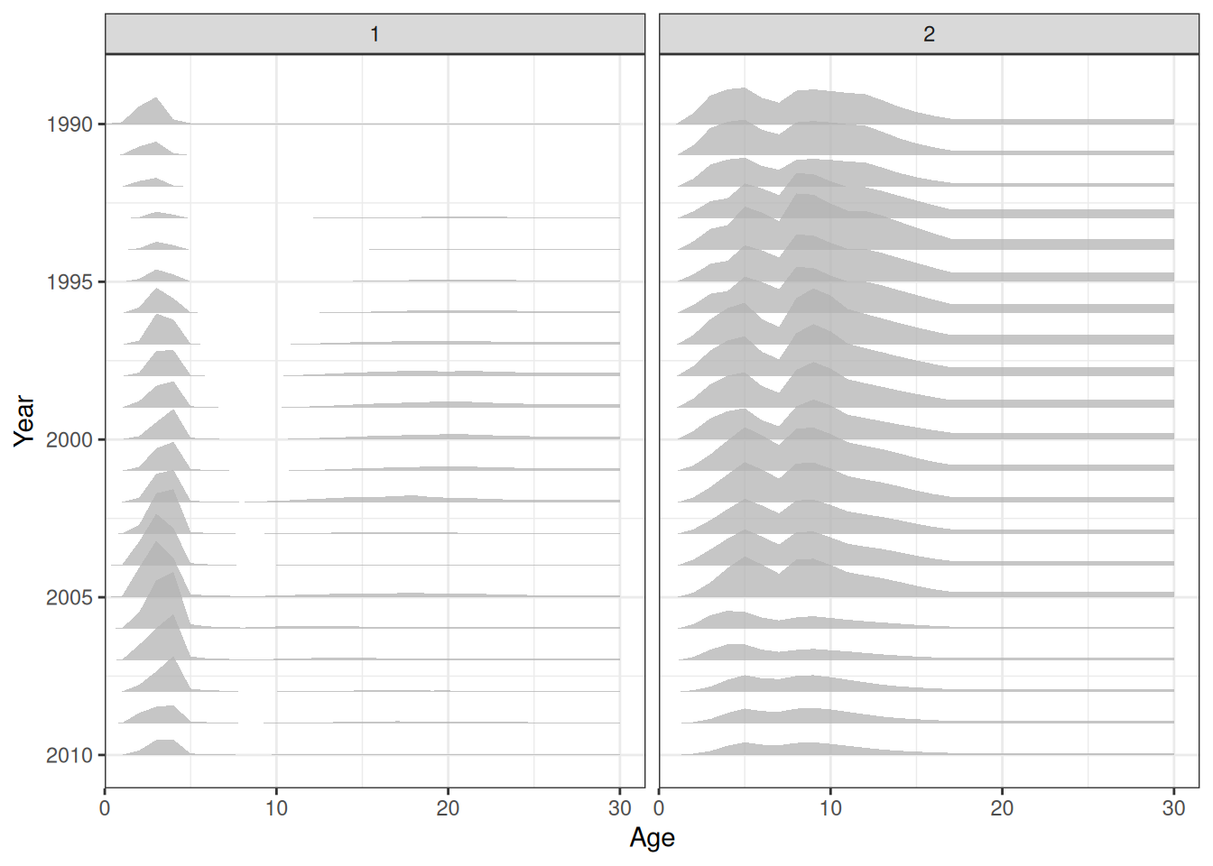
In the plots below, the different coloured blocks of years indicate blocks of parameters, vertical dashed lines indicate the minimum and maximum ages over which selectivity is estimated, and crosses to the left indicate that LF data is available during that year. Selectivity at age by year is shown for the LL1 (Figure 17), LL2 (Figure 18), LL3 (Figure 19), Indonesian (Figure 20), Australian (Figure 21), and CPUE (Figure 22) fleets. Spawning biomass over time is shown in Figure 23.
# yrs <- c(1952, 1953, 1954, seq(1955, 2020, 5), 2021, 2022)
yrs <- c(1952:2022)
plot_selectivity(data = data, object = obj, years = yrs, fisheries = "LL1")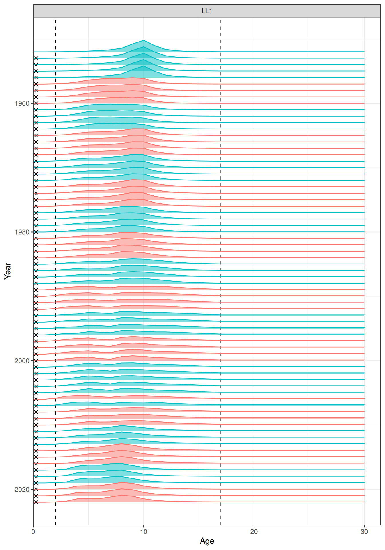
plot_selectivity(data = data, object = obj, years = yrs, fisheries = "LL2")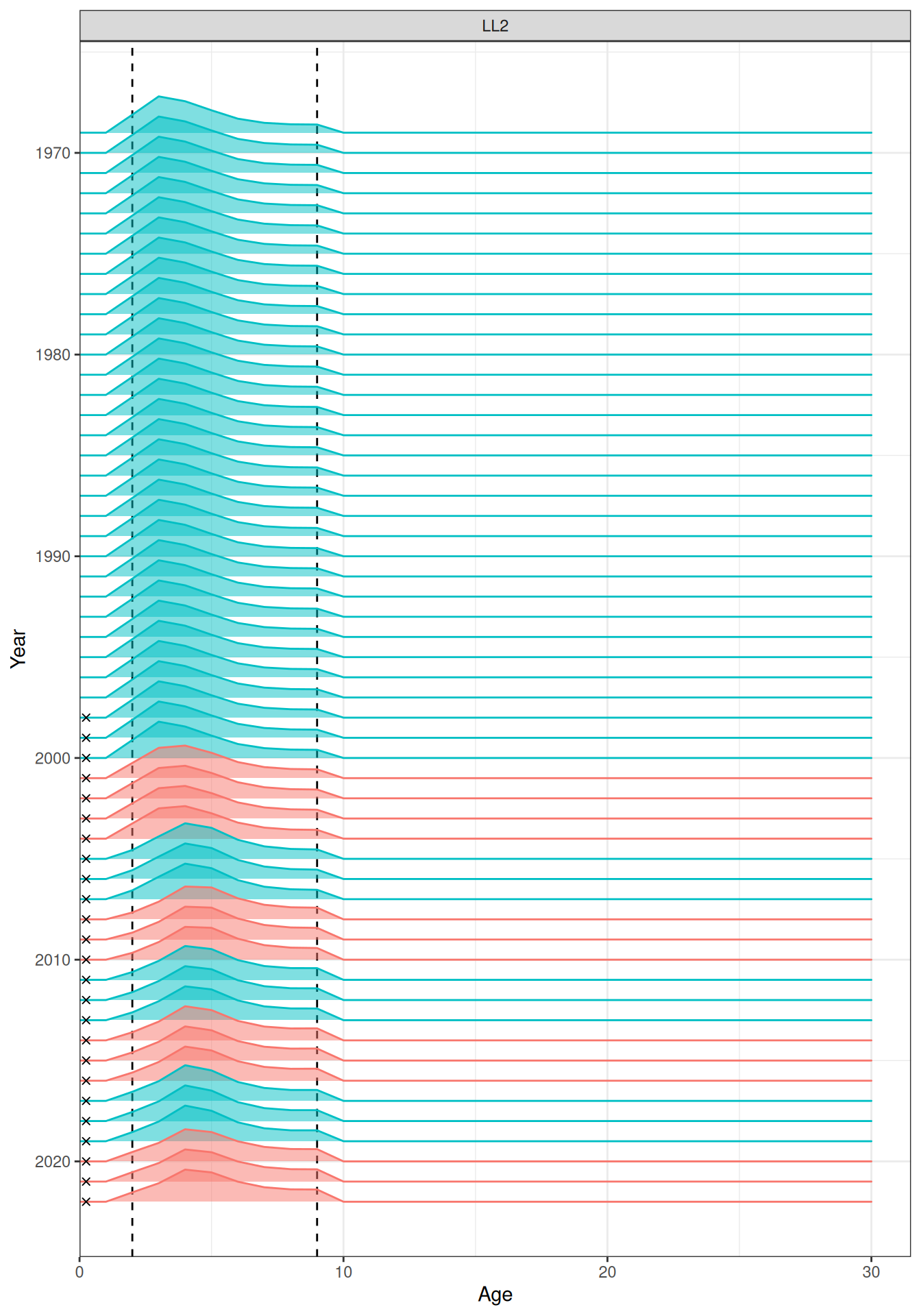
plot_selectivity(data = data, object = obj, years = yrs, fisheries = "LL3")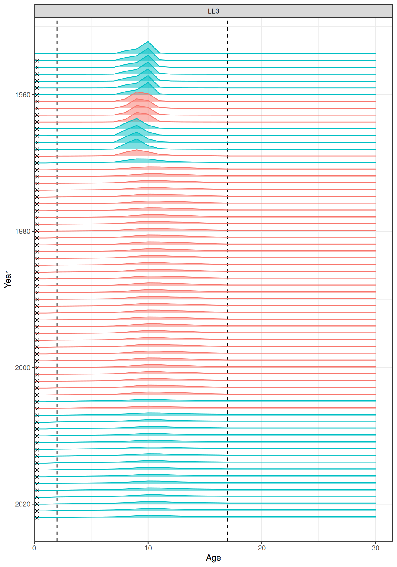
# plot_selectivity(data = data, object = obj, years = yrs, fisheries = "LL4")
plot_selectivity(data = data, object = obj, years = yrs, fisheries = "Indonesian")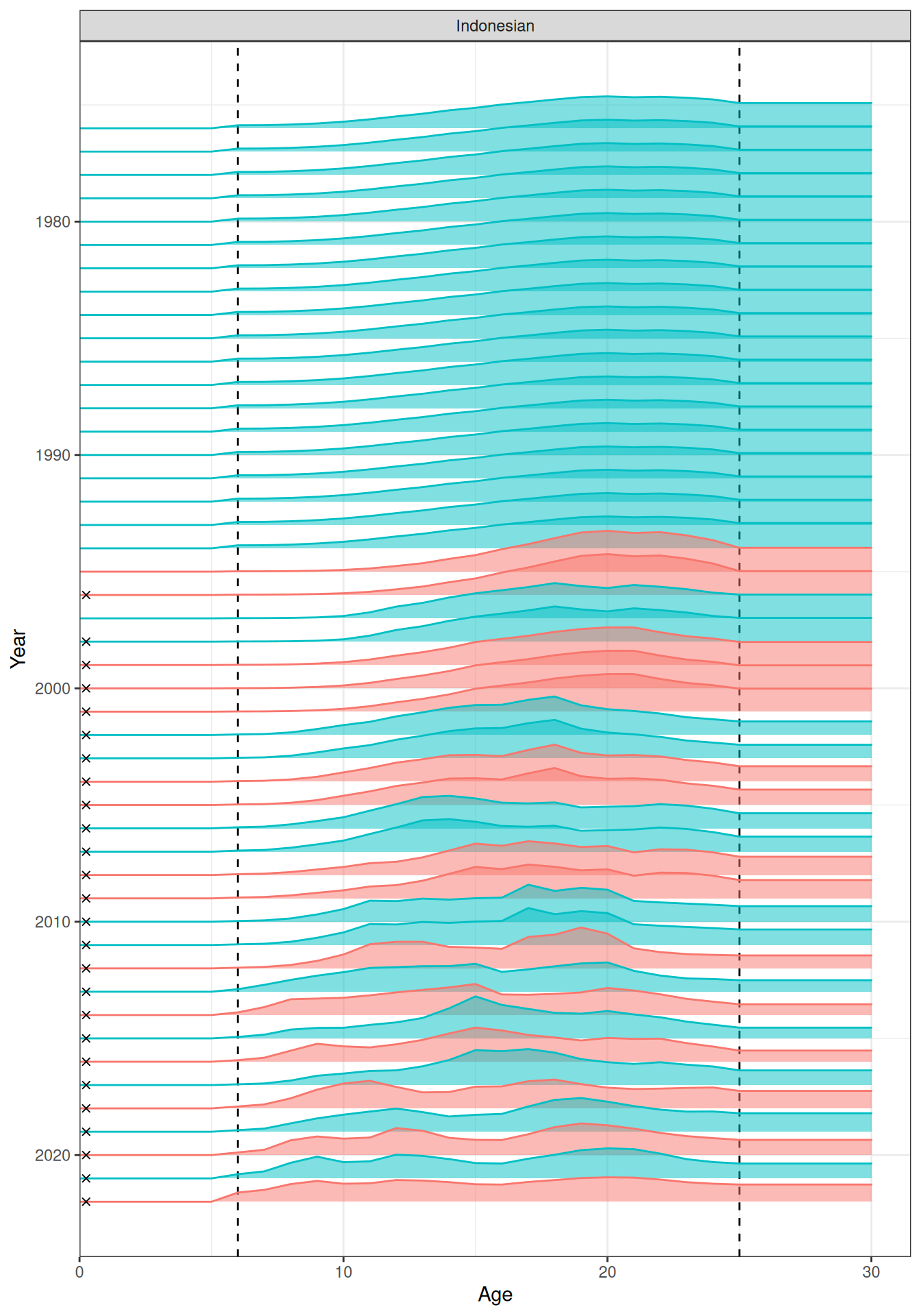
plot_selectivity(data = data, object = obj, years = yrs, fisheries = "Australian")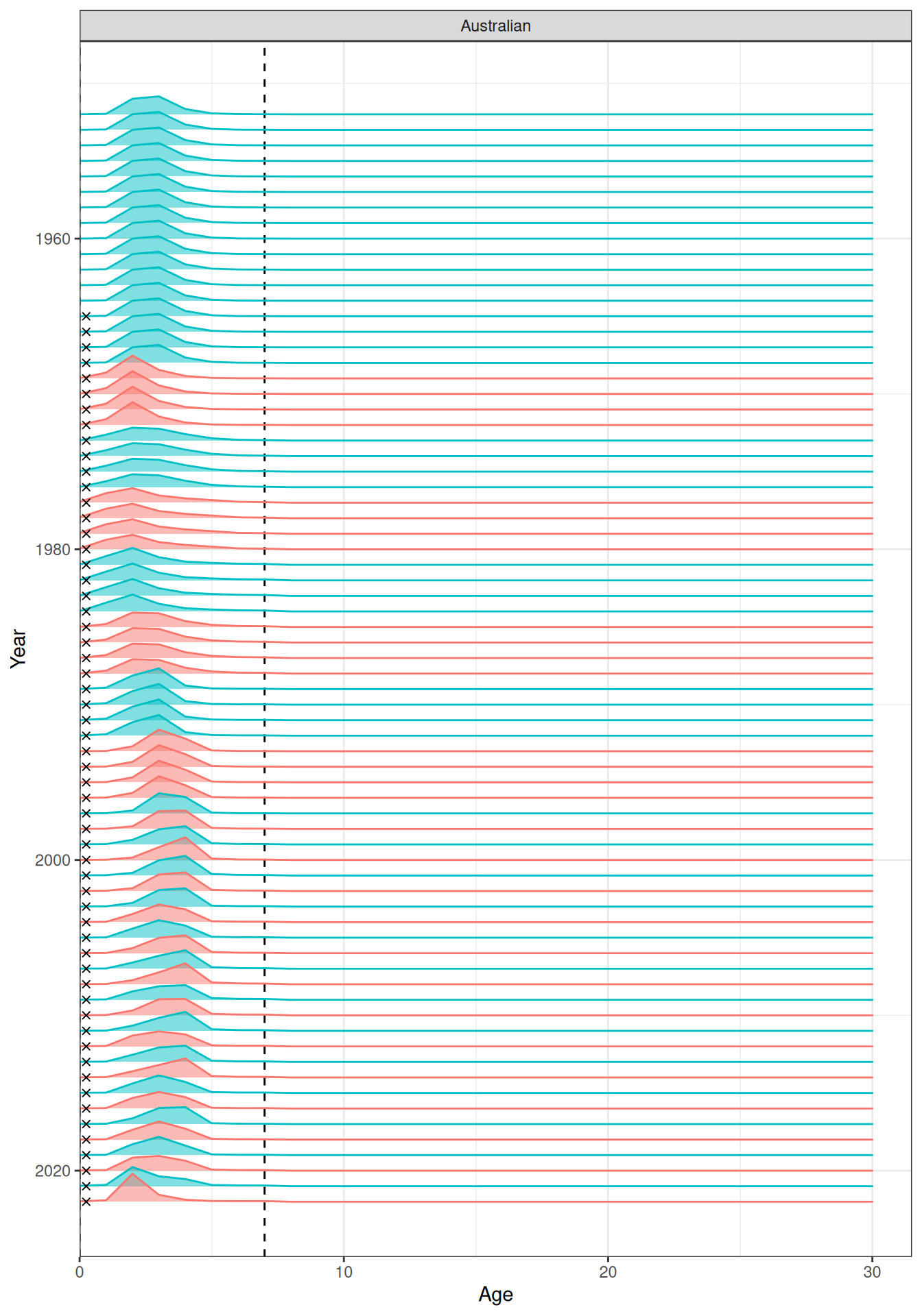
plot_selectivity(data = data, object = obj, years = yrs, fisheries = "CPUE")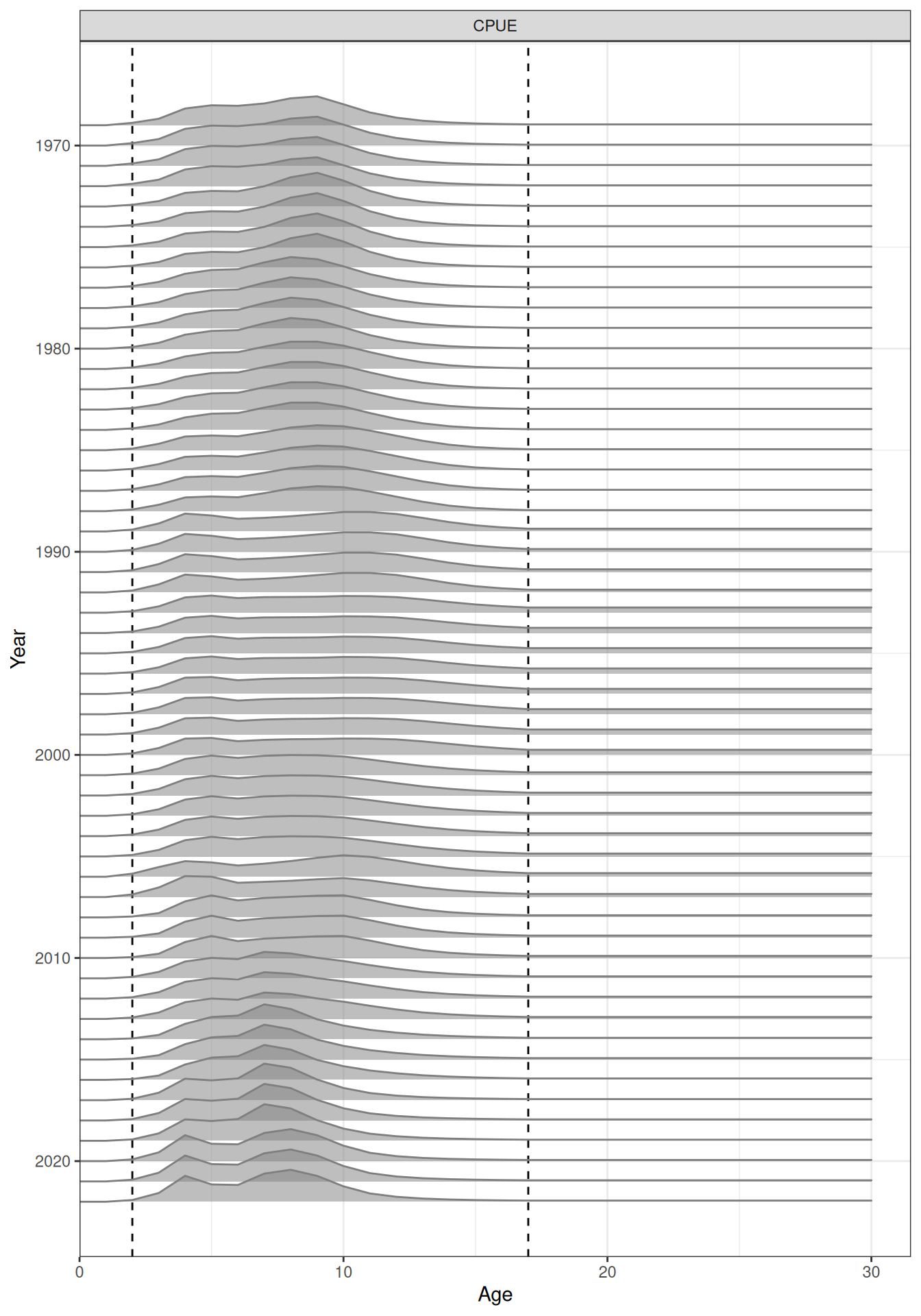
plot_biomass_spawning(data_list = list(data), object_list = list(obj))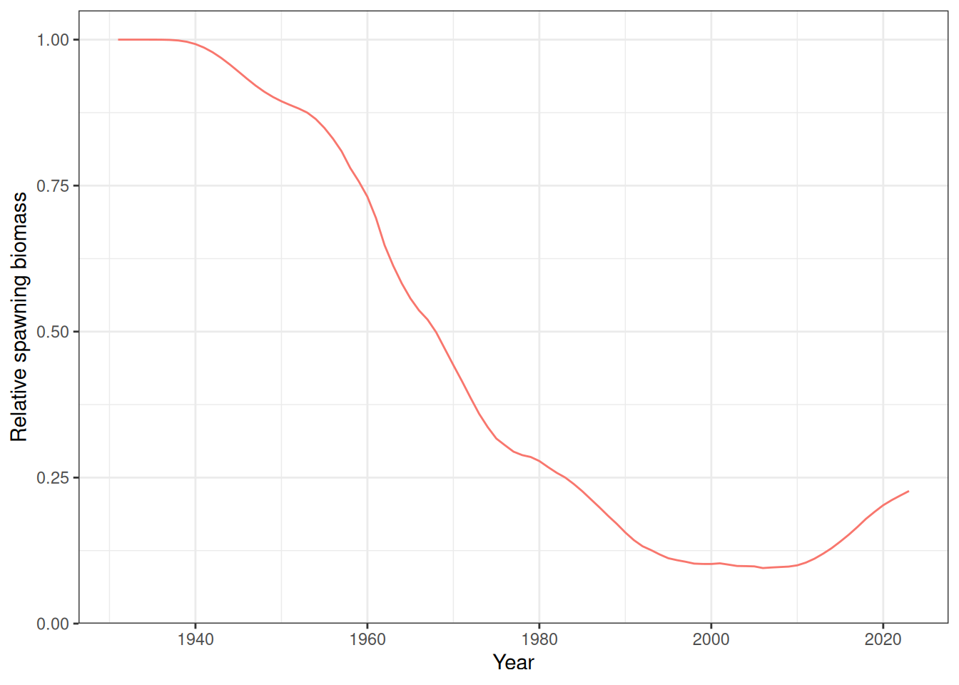
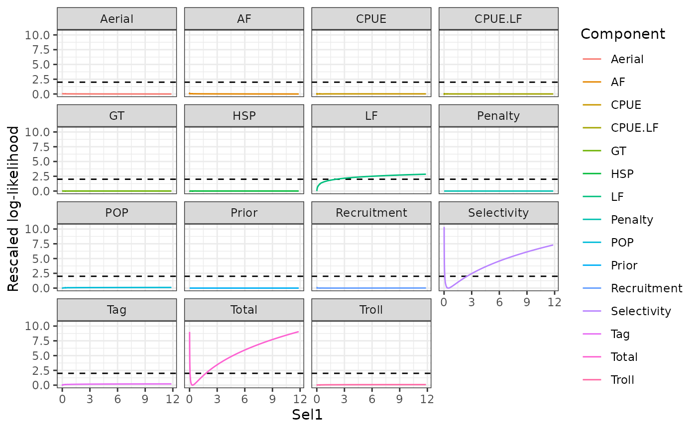
Likelihood profiles
Likelihood profiles can be done for any model parameter using the function sbtprofile. The ytol argument defines the range of likelihood values to explore. A profile can be run using either using name or lincomb arguments, where the latter can be used if there are multiple parameters with the same name (e.g., par_log_sel_1).
# ytol <- 9
# prof_B0 <- sbtprofile(obj = obj, name = "par_log_B0", ytol = ytol)
# prof_m4 <- sbtprofile(obj = obj, name = "par_log_m4", ytol = ytol)
# prof_m30 <- sbtprofile(obj = obj, name = "par_log_m30", ytol = ytol)
# lincomb <- numeric(length(obj$par)); lincomb[6] <- 1
# prof_sel1 <- sbtprofile(obj = obj, lincomb = lincomb, ytol = ytol)
# save(prof_B0, prof_m4, prof_m30, prof_sel1,
#      file = "inst/extdata/profiles.rda")
load(system.file("extdata", "profiles.rda", package = "sbt"))
Note that the profile for B0 did not work very well, likelihood for LFs was zero when B0 was too low. Need to look into this. Profiles are shown for B0 (Figure 24), M4 (Figure 25), M30 (Figure 26), and a selectivity parameter (Figure 27).
head(prof_B0)
obj$env$last.par.best[names(obj$par) == "par_log_B0"]
plot_profile(obj = obj, x = prof_B0 %>% filter(is.finite(value)), xlab = "B0")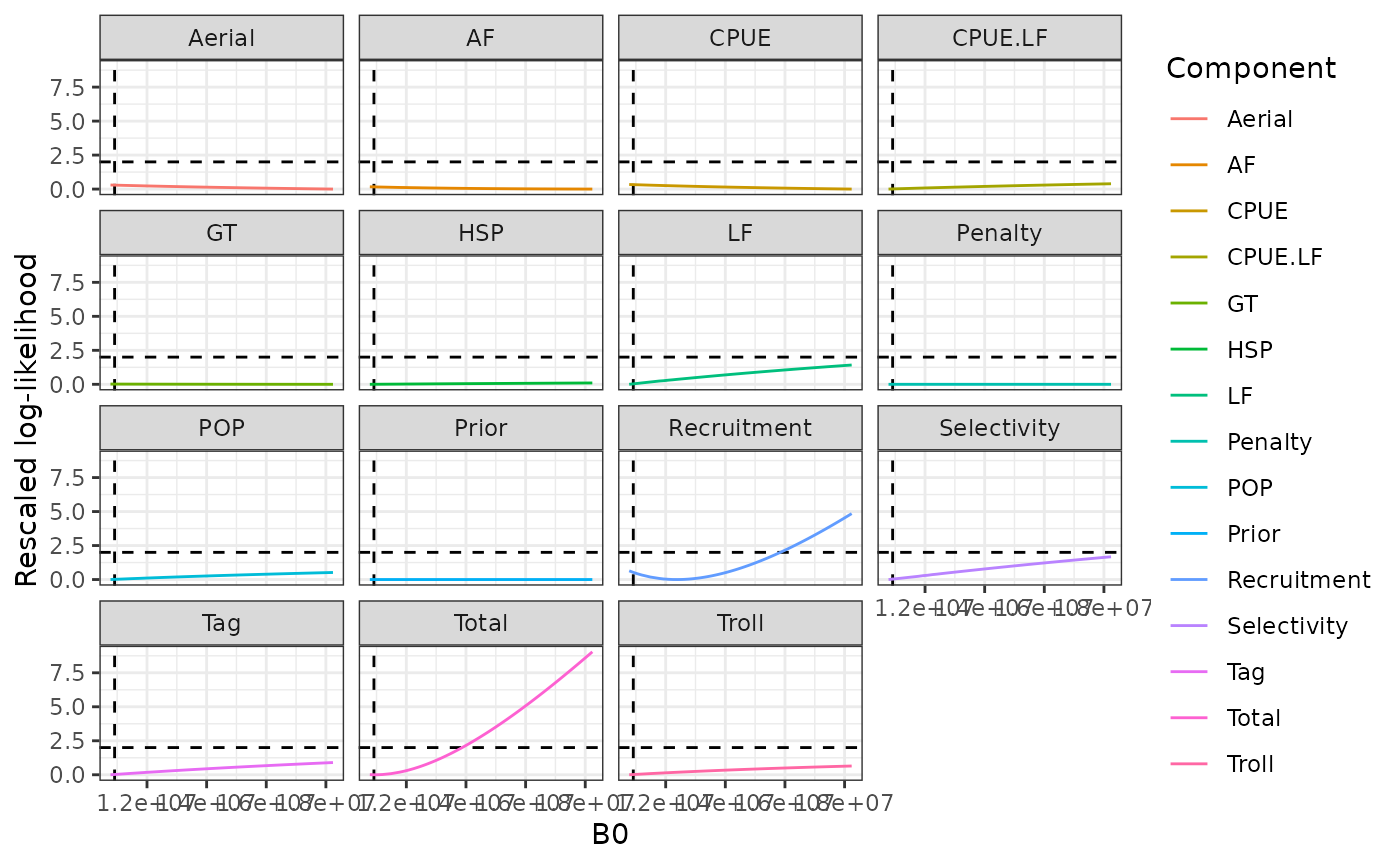
plot_profile(obj = obj, x = prof_m4, xlab = "M4")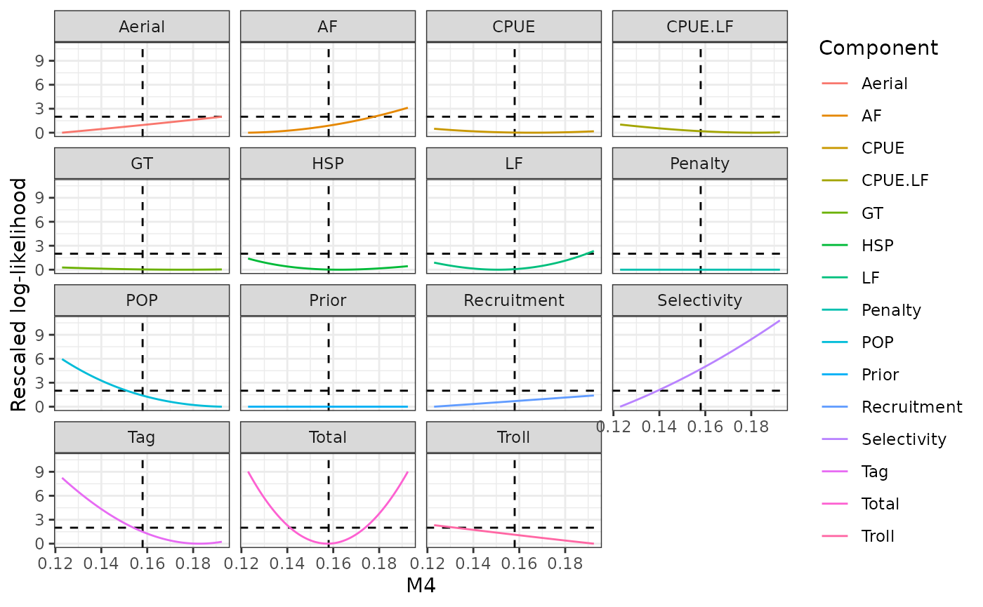
plot_profile(obj = obj, x = prof_m30, xlab = "M30")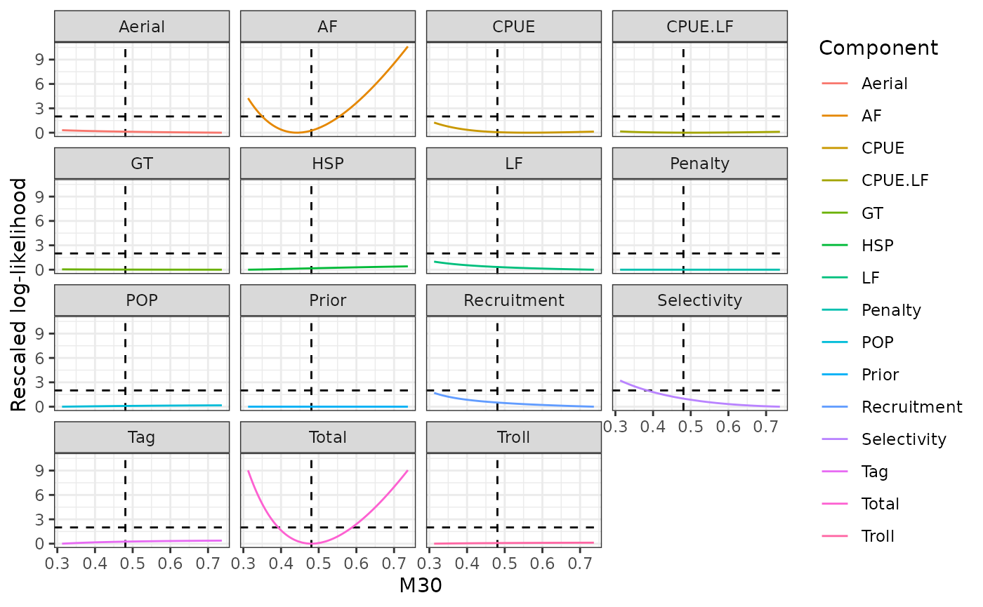
plot_profile(obj = obj, x = prof_sel1, xlab = "Sel1")Warning: Removed 15 rows containing missing values or values outside the scale range
(`geom_vline()`).