Plot CPUE

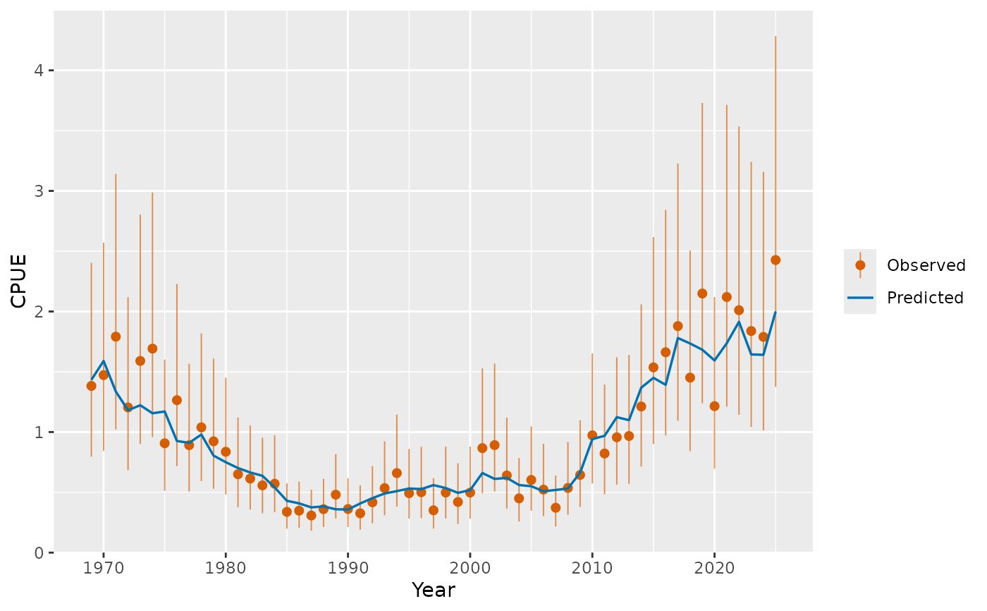
Plot observed and predicted CPUE with approximate lognormal observation intervals.

Usage

plot_cpue(
  fit = NULL,
  object = NULL,
  posterior = NULL,
  probs = c(0.025, 0.975),
  nsim = 0L,
  level = 0.95,
  observed_color = "#D55E00",
  predicted_color = "#0072B2",
  simulated_color = "grey70",
  data = NULL
)

Arguments

fit

An sbt_fit object. Its fitted point estimate is always available; when the fit contains the required embedded posterior summary, posterior = NULL also displays posterior uncertainty.

object

Legacy RTMB objective used only with a legacy data-list input.

posterior

Use NULL to plot the fit's required embedded posterior summary, or FALSE for point estimates only. External posterior objects are not accepted.

probs

A numeric vector of length 2 with probabilities in [0,1] for plotting quantiles of the posterior distribution. Default is c(0.025, 0.975).

nsim

A numeric value specifying the number of simulations to plot. Use 0 to suppress simulated lines. Default is 0.

level

Numeric confidence level for the approximate observation intervals. The default is 0.95.

observed_color

Color used for observed CPUE points and intervals.

predicted_color

Color used for the predicted CPUE line.

simulated_color

Color used for optional simulated CPUE lines.

data

Legacy named alias for a model data list; supply object as well.

Value

A ggplot2 object displaying observed and predicted CPUE by year.

See also

Other diagnostic plots: plot_af(), plot_biomass_spawning(), plot_gt(), plot_hsps(), plot_lf(), plot_pops(), plot_recruitment(), plot_selectivity(), plot_tags(), plot_tags_residuals()

Examples

fit <- sbt_example_fit()
#> Warning: Dependency versions differ: RTMBdist, TMB
#> Warning: Dependency versions differ: RTMBdist, TMB
plot_cpue(fit, posterior = FALSE)