Overview
This vignette demonstrates how to conduct Bayesian inference for the CCSBT stock assessment model using the SparseNUTS package and the sparse inverse Hessian generated by RTMB (https://github.com/noaa-afsc/SparseNUTS). We illustrate the setup, sampling procedure, and posterior diagnostics. If you have not done so already, you will need to install the packages below:
remotes::install_github("janoleko/RTMBdist")
remotes::install_github("andrjohns/StanEstimators")
remotes::install_github("noaa-afsc/SparseNUTS")Markov chain Monte Carlo (MCMC) can be done using the sample_snuts function from the SparseNUTS package.
mcmc <- sample_snuts(
  obj = obj, metric = "auto", init = "last.par.best",
  num_samples = 500, num_warmup = 1000, chains = 4, cores = 4,
  control = list(adapt_delta = 0.999), globals = sbt_globals()
)
This MCMC was split into 4 chains, each with a warm-up of 1000 iterations followed by 500 iterations. This resulted in 2000 posterior samples (i.e., no thinning) for 1553 parameters. This MCMC took 49 minutes to complete.
Diagnostics
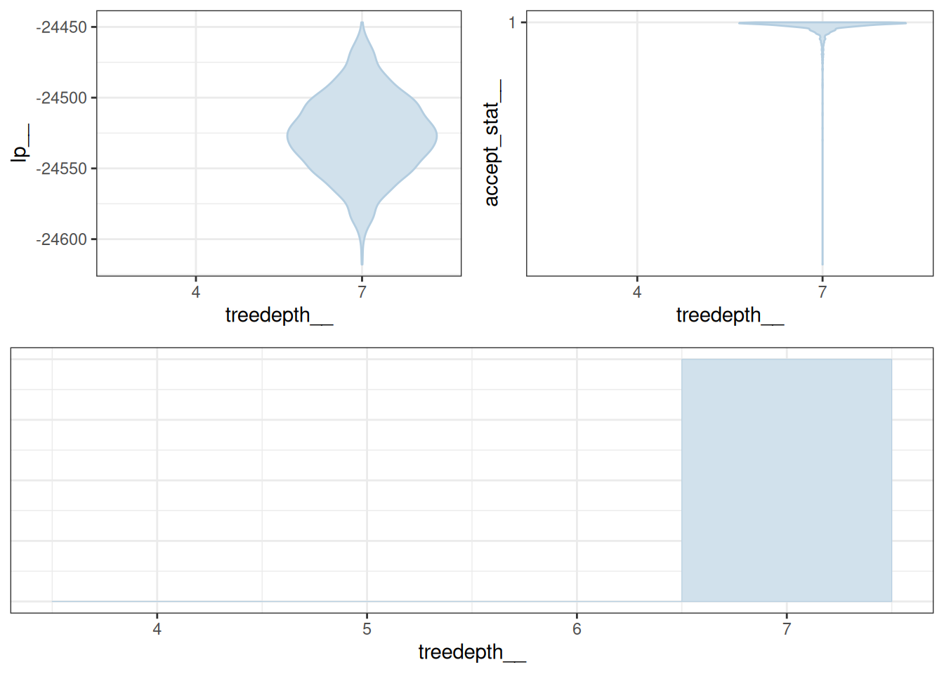
Sampler parameters are shown in Figure 1. A pairs plot for the five slowest mixing parameters is shown in Figure 2. Bayesian and frequentist uncertainty estimates are compared in Figure 3. Marginal distributions are compared in Figure 4. MCMC trace plots are shown in Figure 5. The NUTS energy diagnostic is shown in Figure 6 and additional NUTS diagnostics in Figure 7.
plot_sampler_params(fit = mcmc, plot = TRUE)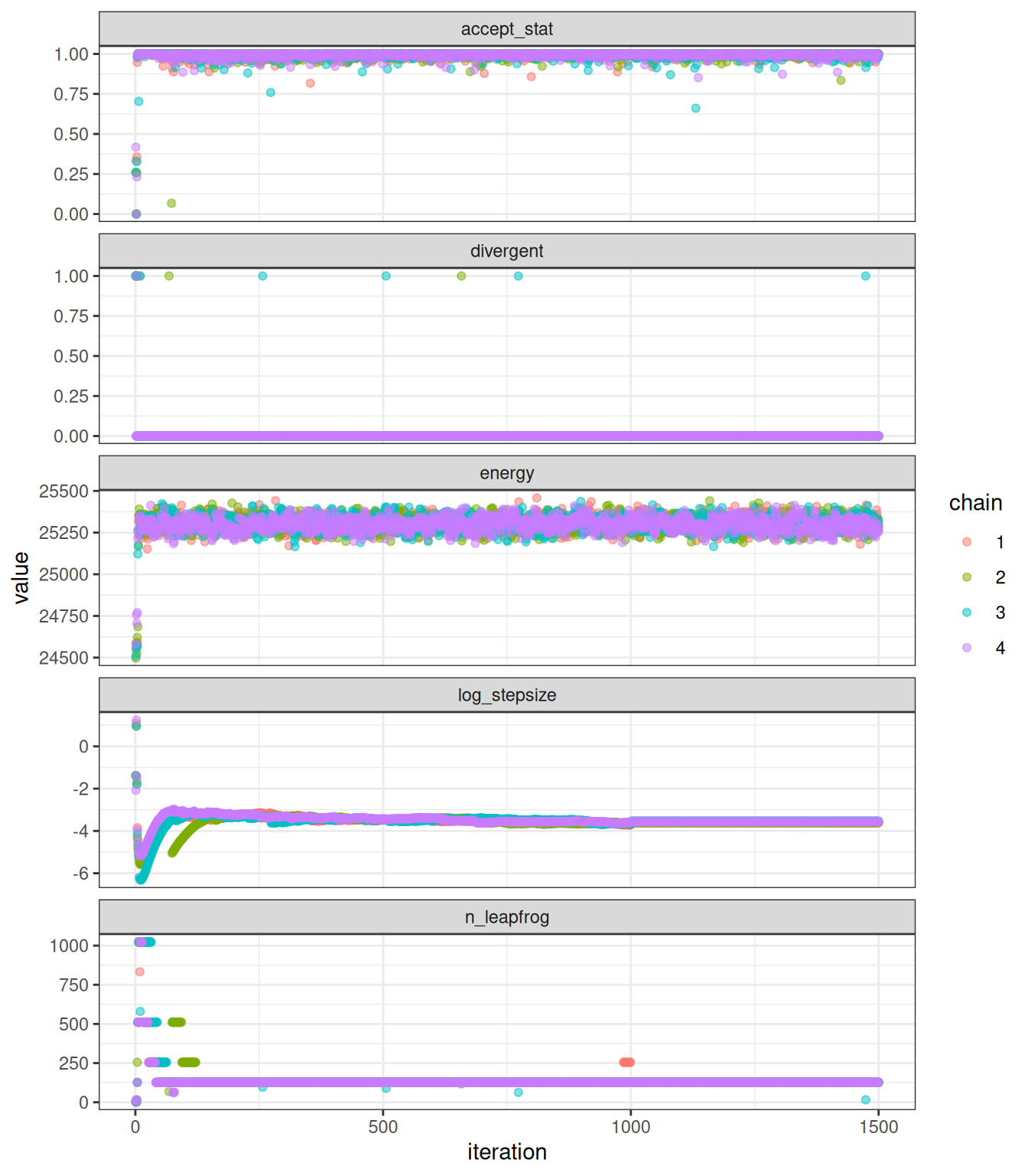
# decamod::pairs_rtmb(fit = mcmc, order = "mismatch", pars = 1:5)
# decamod::pairs_rtmb(fit = mcmc, order = "slow", pars = 1:5)
# decamod::pairs_rtmb(fit = mcmc, order = "fast", pars = 1:5)
# pairs_rtmb(fit = mcmc, order = "divergent", pars = 1:5)
pairs(x = mcmc, order = "slow")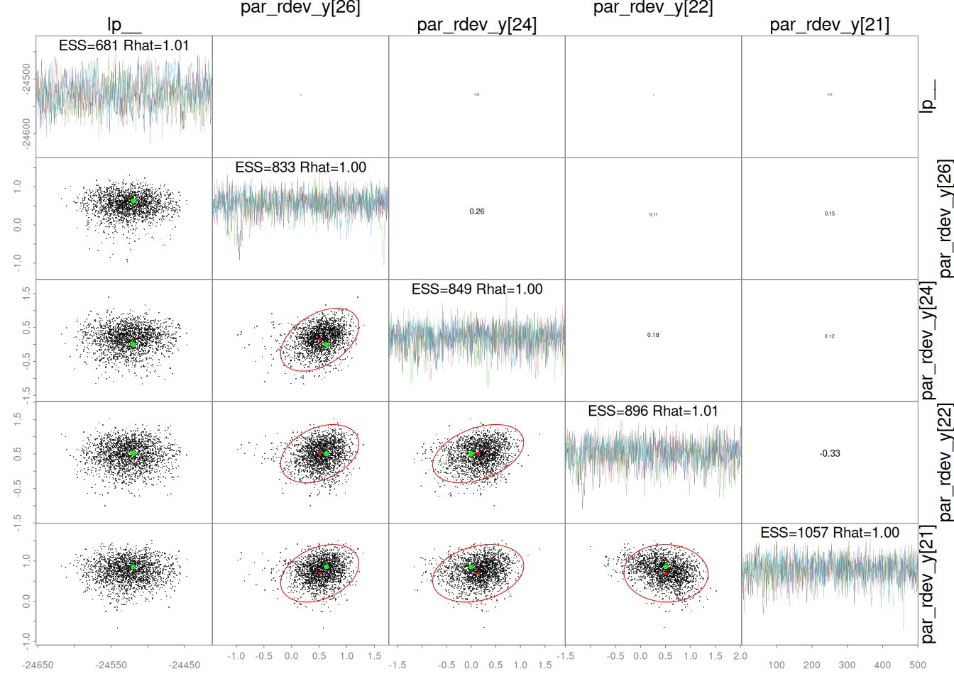
plot_uncertainties(fit = mcmc, log = TRUE, plot = TRUE)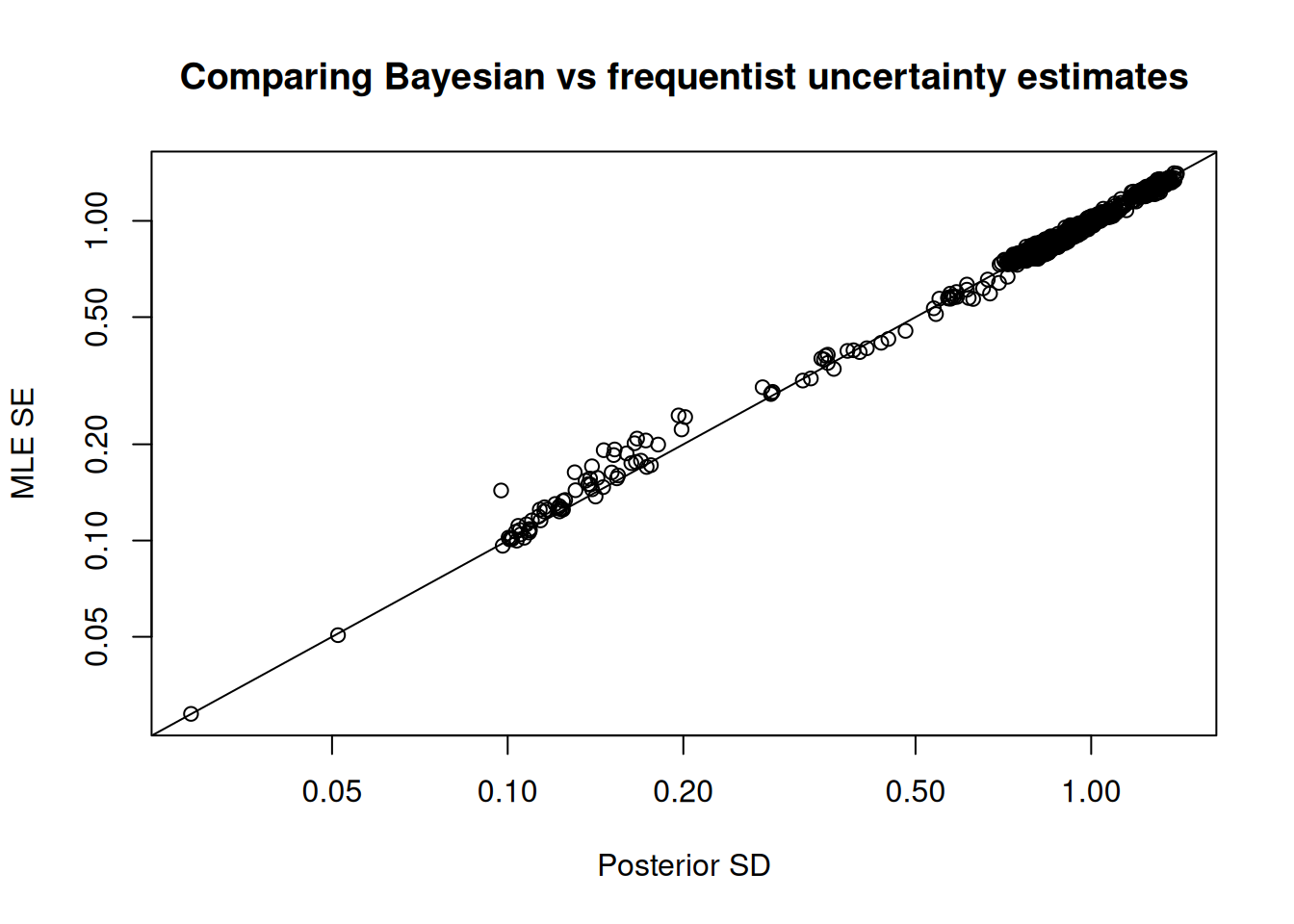
plot_marginals(fit = mcmc, pars = 1:6)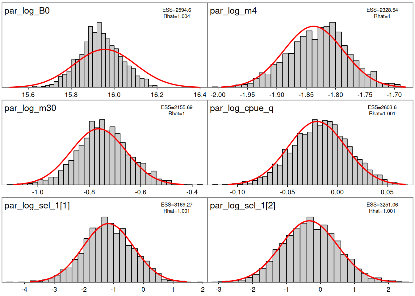
post <- as.data.frame(mcmc)
pars <- mcmc$par_names[1:6]
mcmc_trace(x = post, pars = pars)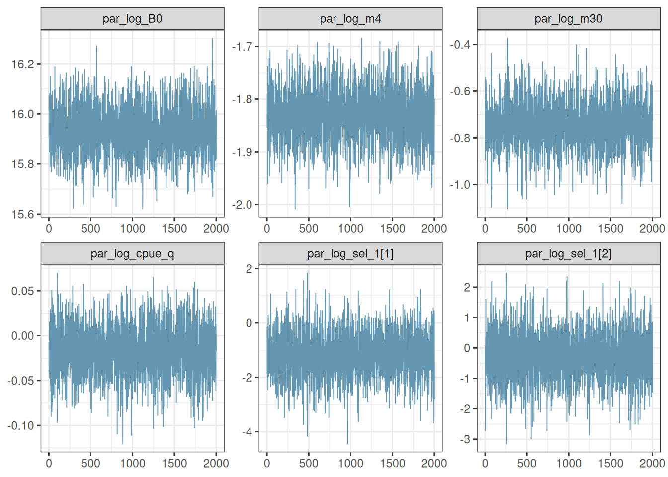
Overlaid histograms showing energy__ vs the change in energy__. See Betancourt (2016) for details.
np <- extract_sampler_params(fit = mcmc) %>%
  pivot_longer(-c(chain, iteration), names_to = "Parameter", values_to = "Value") %>%
  select(Iteration = iteration, Parameter, Value, Chain = chain) %>%
  mutate(Parameter = factor(Parameter), Iteration = as.integer(Iteration), Chain = as.integer(Chain)) %>%
  as.data.frame()

mcmc_nuts_energy(x = np)
`stat_bin()` using `bins = 30`. Pick better value `binwidth`.
`stat_bin()` using `bins = 30`. Pick better value `binwidth`.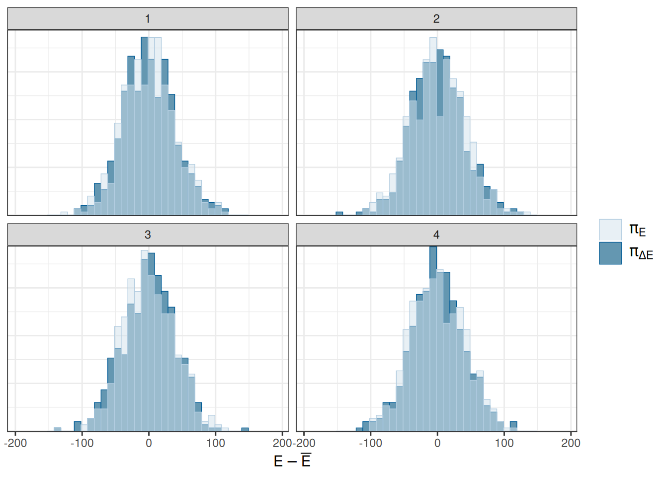
lp <- extract_samples(mcmc, inc_lp = TRUE, as.list = TRUE) %>%
  melt(value.name = "Value") %>%
  filter(Var2 == "lp__") %>%
  mutate(Chain = as.integer(L1), Iteration = as.integer(Var1)) %>%
  select(Chain, Iteration, Value)
mcmc_nuts_acceptance(x = np, lp = lp)
`stat_bin()` using `bins = 30`. Pick better value `binwidth`.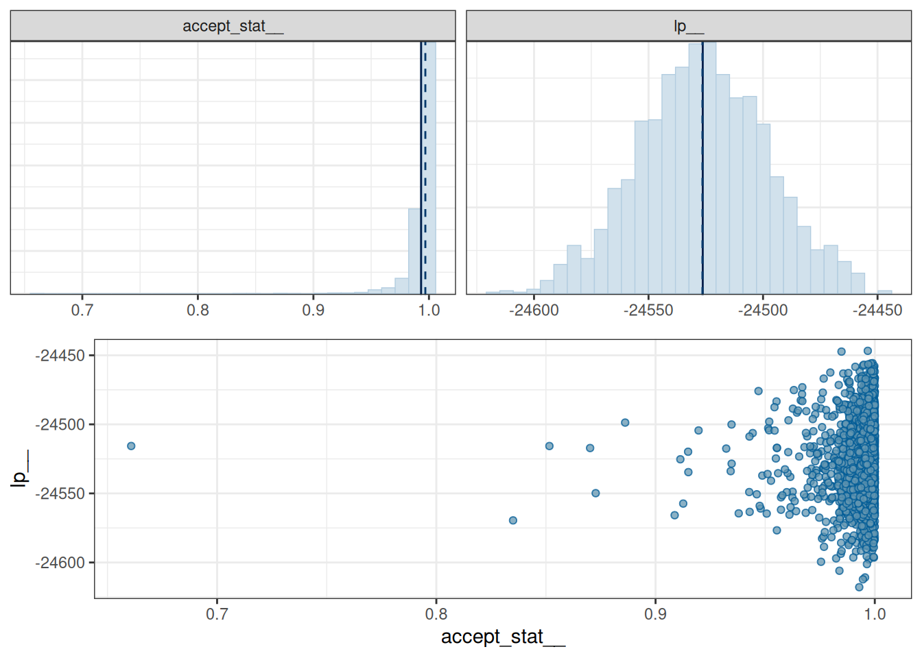
mcmc_nuts_divergence(x = np, lp = lp)Warning: Groups with fewer than two datapoints have been dropped.
ℹ Set `drop = FALSE` to consider such groups for position adjustment purposes.
Groups with fewer than two datapoints have been dropped.
ℹ Set `drop = FALSE` to consider such groups for position adjustment purposes.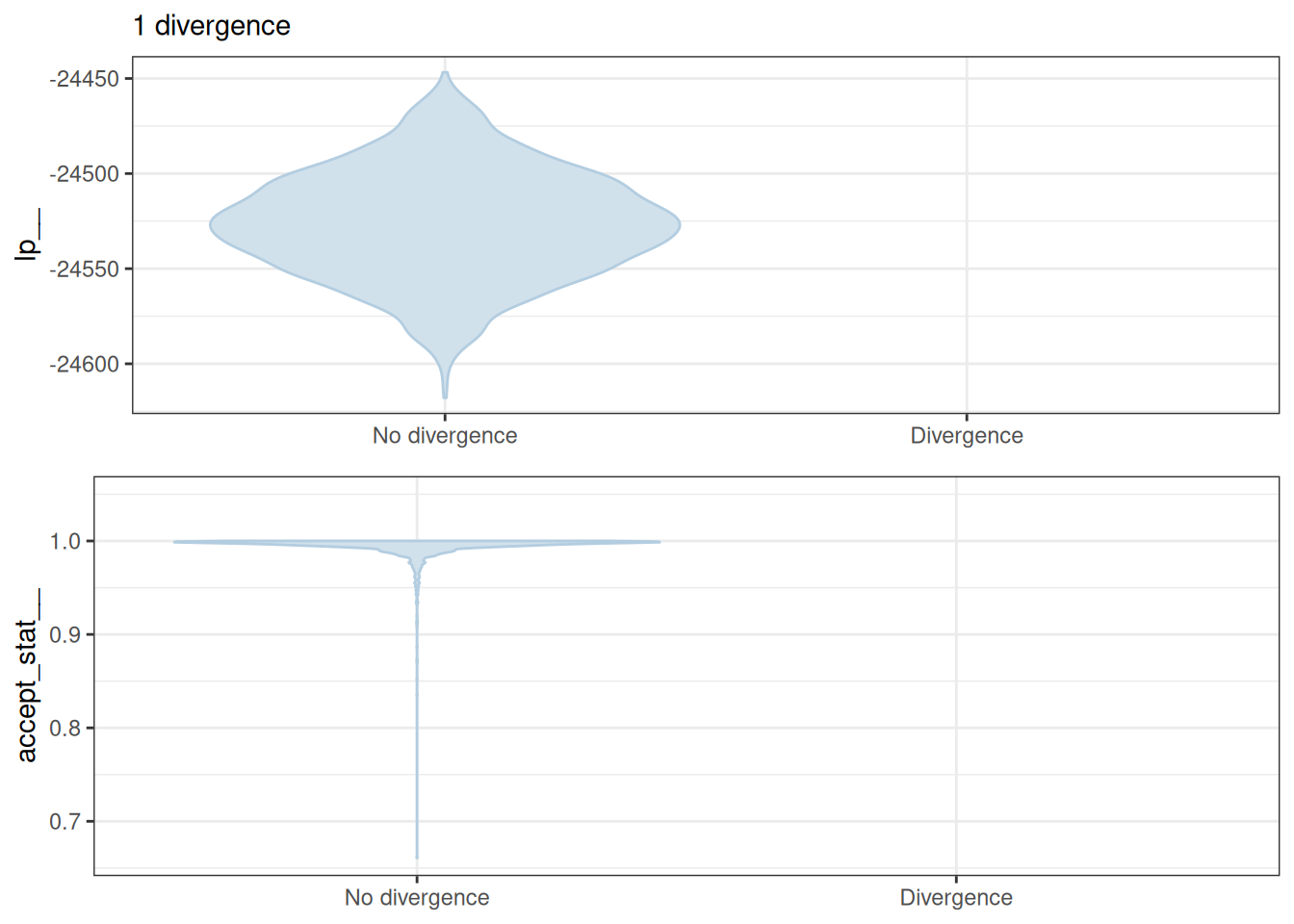
mcmc_nuts_stepsize(x = np, lp = lp)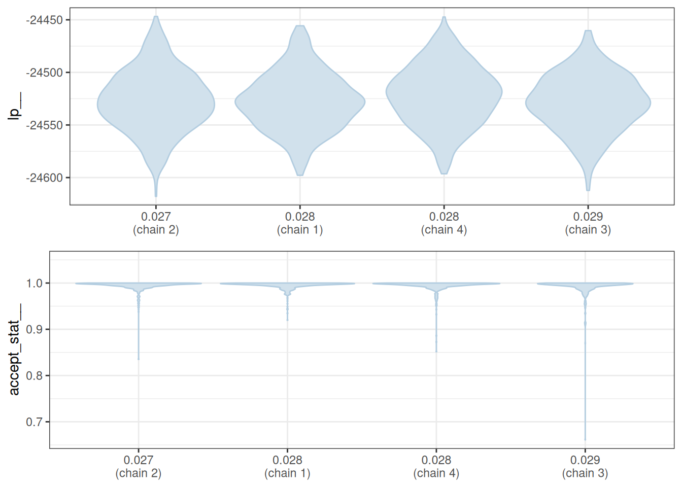
mcmc_nuts_treedepth(x = np, lp = lp)Warning: Groups with fewer than two datapoints have been dropped.
ℹ Set `drop = FALSE` to consider such groups for position adjustment purposes.
Groups with fewer than two datapoints have been dropped.
ℹ Set `drop = FALSE` to consider such groups for position adjustment purposes.
Notes and Next Steps
- Adjust
parsinpairs_rtmb()to inspect specific parameter blocks. - If convergence is slow reduce
adapt_delta. - If divergent transitions persist, increase
warmup,adapt_delta, or use block-wise adaptation. - Consider thinning for large posterior draws before plotting.