
if (dir.exists(file.path("..", "R")) && requireNamespace("pkgload", quietly = TRUE)) {
  pkgload::load_all("..", quiet = TRUE)
} else {
  library(decamod)
}
library(ggplot2)

theme_set(theme_bw())
set.seed(123)

normal_to_lognormal <- function(normmean, normsd) {
  phi <- sqrt(normsd^2 + normmean^2)
  lognorm_meanlog <- log(normmean^2 / phi)
  lognorm_sdlog <- sqrt(log(phi^2 / normmean^2))
  list(meanlog = lognorm_meanlog, sdlog = lognorm_sdlog)
}

find_lognormal_sd <- function(median, sd) {
  mu <- log(median)
  f <- function(sigma2) {
    sqrt((exp(sigma2) - 1) * exp(2*mu + sigma2)) - sd
  }
  sigma2 <- uniroot(f, lower = 1e-8, upper = 100)$root
  return(sqrt(sigma2))
}

Nsim <- 1e5

parameters <- list(
  log_F0 = log(1e-6), logit_U0 = qlogis(1e-10),
  log_R0 = log(237000), log_Rsigma = log(0.4), Rrho = 0.1,
  log_Rmu = log(32), log_Rsd = log(2),
  log_Ma = log(0.107031),
  log_galpha = log(c(16.5524, 18.2545)),
  logit_gdiff = qlogis(c(0.157653, 0.068249)),
  log_gshape = log(c(3.18023, 5.26284)),
  log_gcv = log(c(0.390413, 0.753572)),
  log_gobs = log(0.670252), log_gdd = log(0),
  log_sel50 = log(c(55, 55, 55, 55, 55, 55)),
  log_sel95 = log(c(11, 16, 11, 16, 11, 16)),
  log_selmax = log(c(mean(c(1, 0.735895)),
                     mean(c(0.613501, 0.413777)),
                     1,
                     0.413777,
                     0.735895,
                     0.607853))
)Default prior distributions are specified for all model parameters following the approach described in Quinn and Deriso (1999) and Hilborn and Walters (1992), with lognormal priors used for positive-valued parameters (Kristensen et al. 2016).
priors <- list()
priors[["logit_U0"]] <- list(type = "normal", par1 = 0, par2 = 1.5, index = which("logit_U0" == names(parameters)))
priors[["log_Ma"]] <- list(type = "normal", par1 = log(0.12), par2 = 0.4, index = which("log_Ma" == names(parameters)))
priors[["log_galpha"]] <- list(type = "normal", par1 = log(2), par2 = 1.655705, index = which("log_galpha" == names(parameters))) # matches dnorm(2, 30)
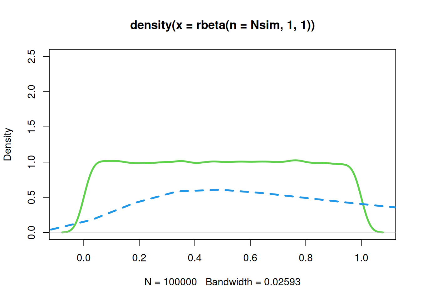
# plot(density(plogis(rnorm(1e6, -2, 1.5))))
# lines(density(rbeta(1e6, 1, 6)))
priors[["logit_gdiff"]] <- list(type = "normal", par1 = -2, par2 = 1.5, index = which("logit_gdiff" == names(parameters)))
priors[["log_gshape"]] <- list(type = "normal", par1 = c(log(4.81), log(4.51)), par2 = c(0.2016748, 0.2142224), index = which("log_gshape" == names(parameters))) # matches dnorm(4.81, 1), dnorm(4.51, 1)
priors[["log_gcv"]] <- list(type = "normal", par1 = c(log(0.59), log(0.82)), par2 = c(0.439544, 0.3360953), index = which("log_gcv" == names(parameters))) # matches dnorm(0.59, 0.3), dnorm(0.82, 0.3)
priors[["log_gobs"]] <- list(type = "normal", par1 = log(1.48), par2 = 0.04990982, index = which("log_gobs" == names(parameters))) # matches dnorm(1.48, 0.074)
priors[["log_Rmu"]] <- list(type = "normal", par1 = log(32), par2 = 0.1, index = which("log_Rmu" == names(parameters)))
priors[["log_Rsd"]] <- list(type = "normal", par1 = log(2), par2 = 0.1, index = which("log_Rsd" == names(parameters)))
priors[["log_Rsigma"]] <- list(type = "normal", par1 = log(0.4), par2 = 0.3, index = which("log_Rsigma" == names(parameters)))
priors[["log_sel50"]] <- list(type = "normal", par1 = log(50), par2 = 0.5, index = which("log_sel50" == names(parameters))) # matches dnorm(50, 30)
priors[["log_sel95"]] <- list(type = "normal", par1 = log(10), par2 = 1.124519, index = which("log_sel95" == names(parameters))) # matches dnorm(10, 30)
priors[["log_selmax"]] <- list(type = "normal", par1 = -log(2) / 2, par2 = sqrt(log(2)), index = which("log_selmax" == names(parameters)))

evaluate_priors(parameters, priors)
#> [1] -261.5602
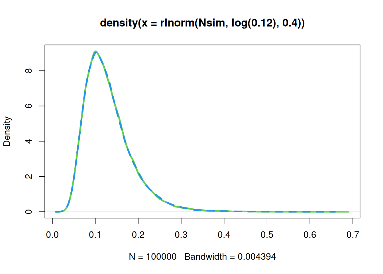
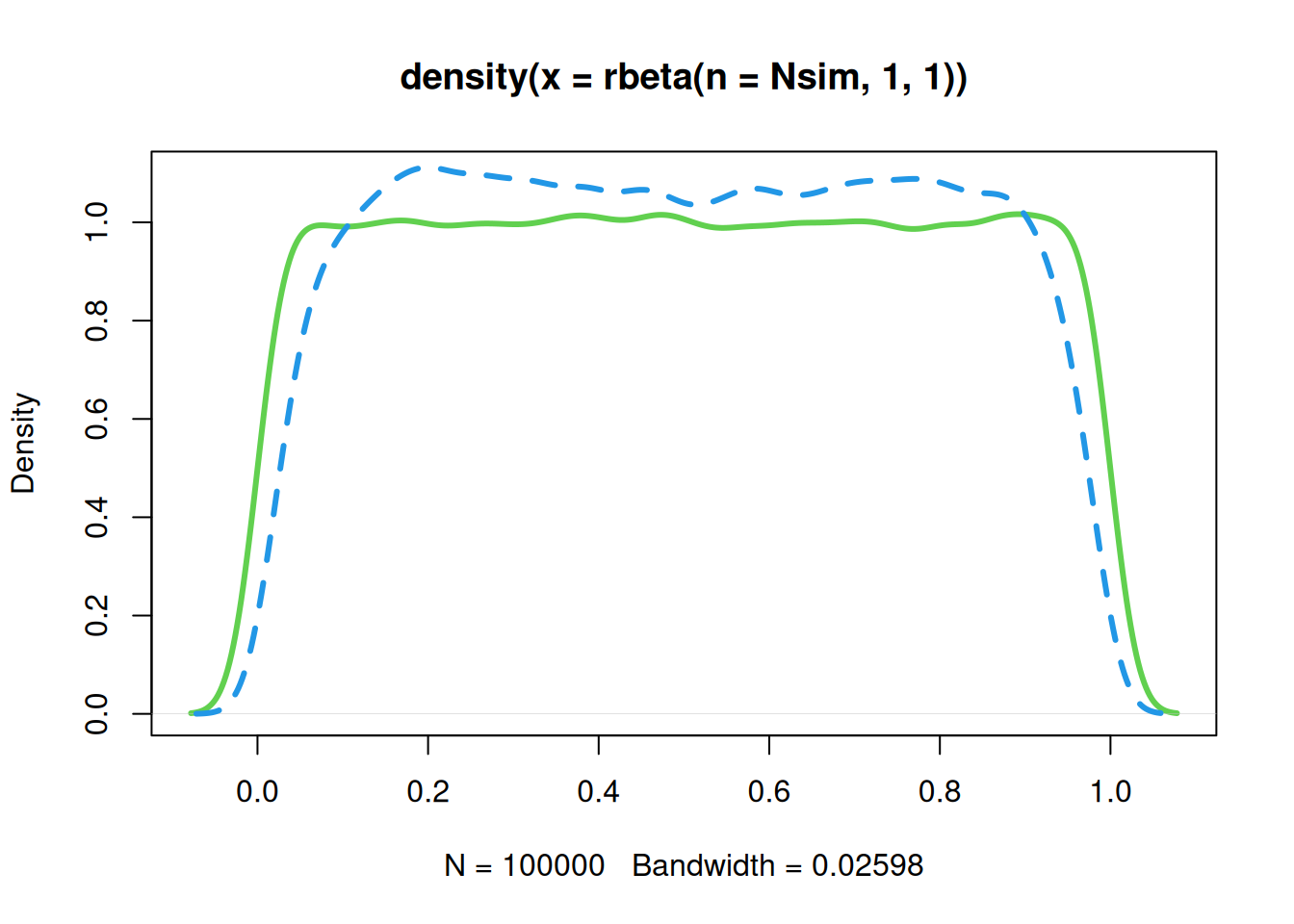
Green is the original prior; blue is the transformed prior candidate.
Natural mortality (M)
The prior distribution for natural mortality () is informed by meta-analyses and life-history theory (Clark 1999; Quinn and Deriso 1999).
U0 and gdiff
galpha
mu <- 2
sig <- 30
# sig <- 3
(sdlog <- find_lognormal_sd(mu, sig))
#> [1] 1.655705
y1 <- rnorm(n = Nsim, mean = mu, sd = sig)
y2 <- exp(rnorm(n = Nsim, log(mu), sdlog))
summary(y1)
#>     Min.  1st Qu.   Median     Mean  3rd Qu.     Max.
#> -128.341  -18.405    1.787    1.824   22.093  125.153
summary(y2)
#>      Min.   1st Qu.    Median      Mean   3rd Qu.      Max.
#>    0.0013    0.6617    2.0206    7.8644    6.1078 3399.1396
plot(density(y1), col = 3, lwd = 3, ylim = c(0, 1))
lines(density(y2), col = 4, lwd = 3, lty = 2)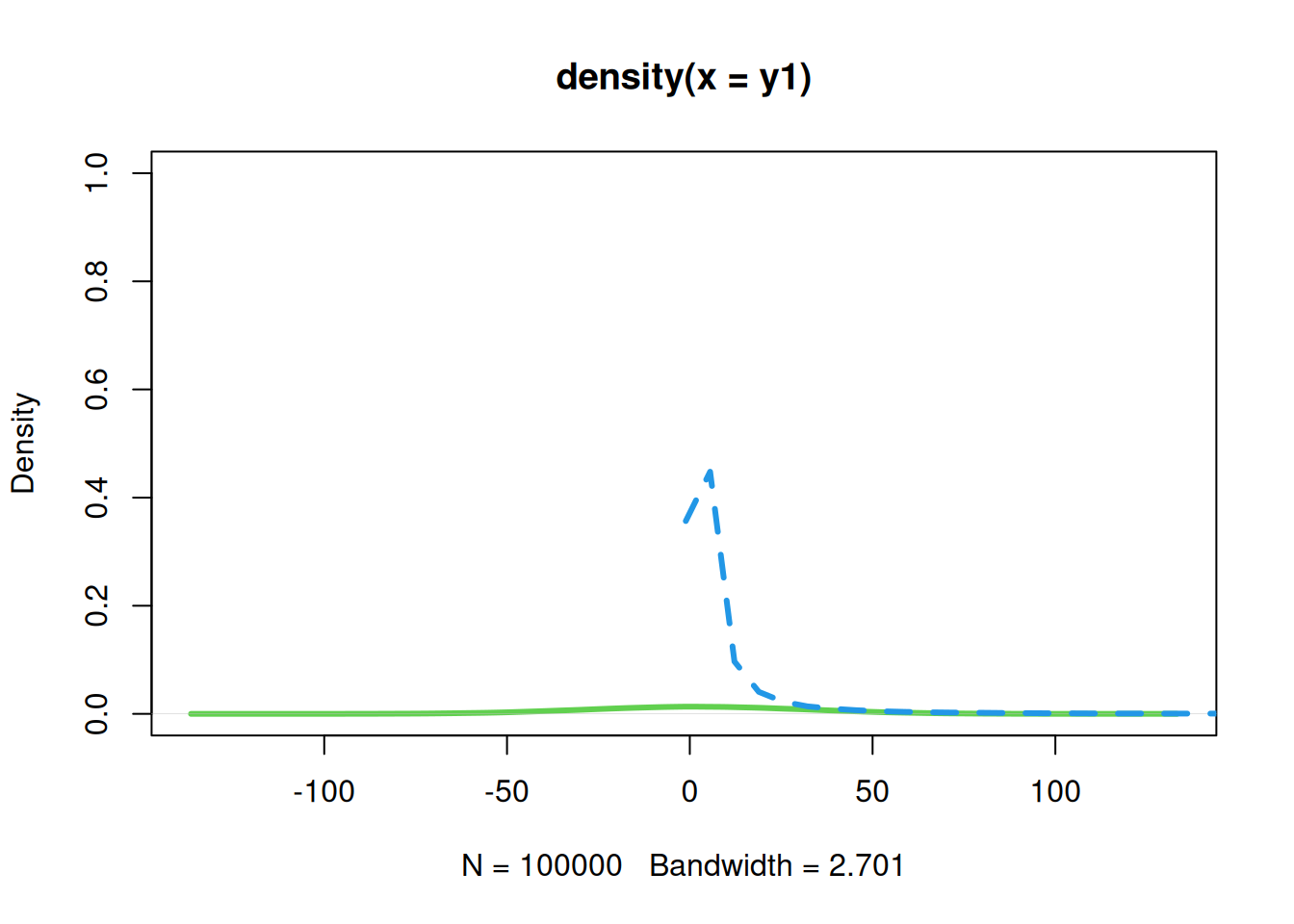
gshape
mu <- 4.81
sig <- 1
(sdlog <- find_lognormal_sd(mu, sig))
#> [1] 0.2016748
y1 <- rnorm(n = Nsim, mean = mu, sd = sig)
y2 <- exp(rnorm(n = Nsim, log(mu), sdlog))
summary(y1)
#>    Min. 1st Qu.  Median    Mean 3rd Qu.    Max.
#> 0.01081 4.13489 4.80784 4.80614 5.48083 9.66077
summary(y2)
#>    Min. 1st Qu.  Median    Mean 3rd Qu.    Max.
#>   1.953   4.197   4.807   4.907   5.512  11.310
plot(density(y1), col = 3, lwd = 3, ylim = c(0, 0.43))
lines(density(y2), col = 4, lwd = 3, lty = 2)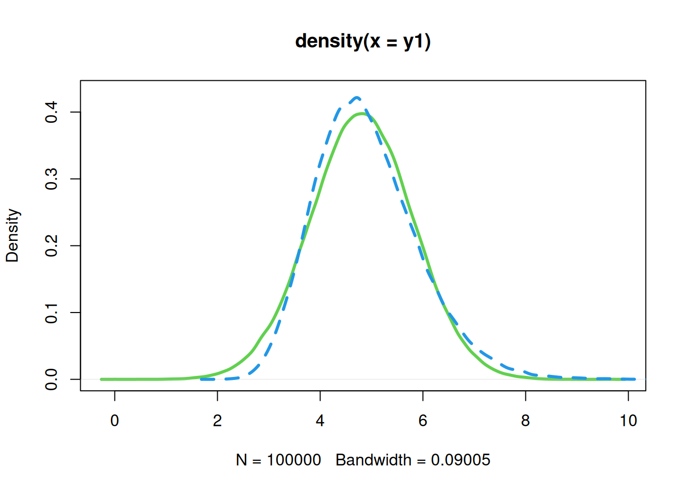
mu <- 4.51
sig <- 1
(sdlog <- find_lognormal_sd(mu, sig))
#> [1] 0.2142224
y1 <- rnorm(n = Nsim, mean = mu, sd = sig)
y2 <- exp(rnorm(n = Nsim, log(mu), sdlog))
summary(y1)
#>    Min. 1st Qu.  Median    Mean 3rd Qu.    Max.
#>  0.4122  3.8294  4.5091  4.5052  5.1794  8.5962
summary(y2)
#>    Min. 1st Qu.  Median    Mean 3rd Qu.    Max.
#>   1.703   3.906   4.510   4.614   5.210  12.393
plot(density(y1), col = 3, lwd = 3, ylim = c(0, 0.43))
lines(density(y2), col = 4, lwd = 3, lty = 2)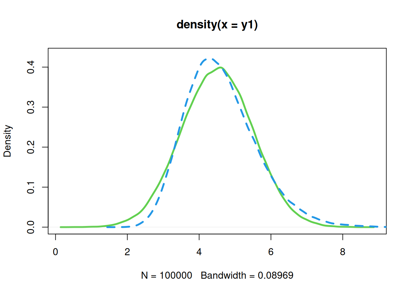
gcv
mu <- 0.59
sig <- 0.3
(sdlog <- find_lognormal_sd(mu, sig))
#> [1] 0.439544
# pp <- normal_to_lognormal(normmean = mu, normsd = sig)
y1 <- rnorm(n = Nsim, mean = mu, sd = sig)
y2 <- exp(rnorm(n = Nsim, log(mu), sdlog))
# y3 <- exp(rnorm(n = Nsim, pp[[1]], pp[[2]]))
summary(y1)
#>    Min. 1st Qu.  Median    Mean 3rd Qu.    Max.
#> -0.7874  0.3877  0.5894  0.5892  0.7893  1.7973
summary(y2)
#>    Min. 1st Qu.  Median    Mean 3rd Qu.    Max.
#> 0.09246 0.43853 0.58849 0.64996 0.79298 3.70429
plot(density(y1), col = 3, lwd = 3, ylim = c(0, 1.6))
lines(density(y2), col = 4, lwd = 3, lty = 2)
# lines(density(y3), col = 5, lwd = 3, lty = 2)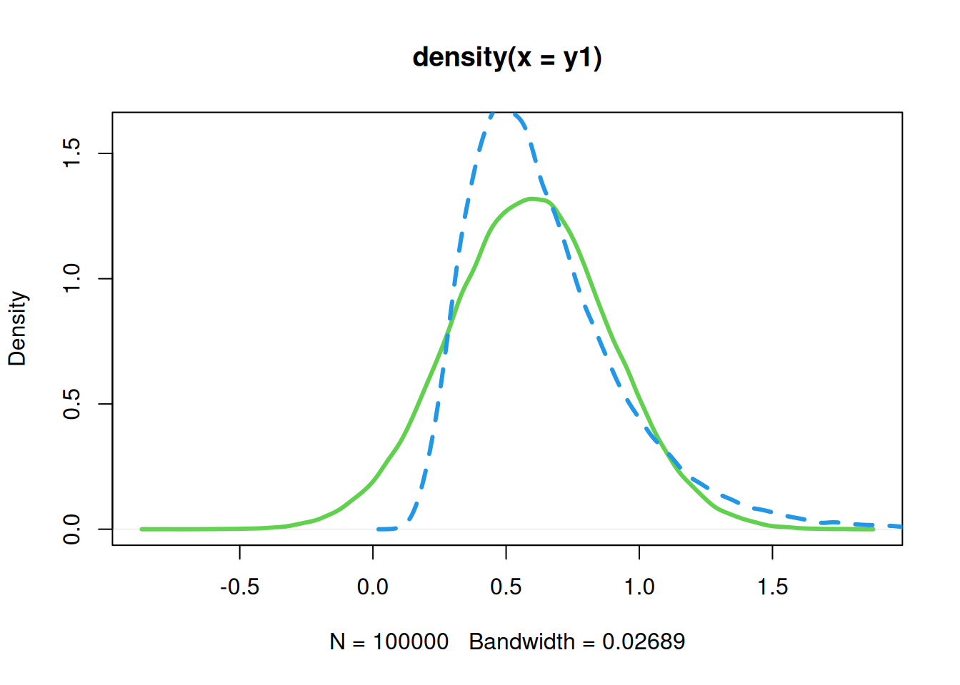
mu <- 0.82
sig <- 0.3
(sdlog <- find_lognormal_sd(mu, sig))
#> [1] 0.3360953
y1 <- rnorm(n = Nsim, mean = mu, sd = sig)
y2 <- exp(rnorm(n = Nsim, log(mu), sdlog))
summary(y1)
#>    Min. 1st Qu.  Median    Mean 3rd Qu.    Max.
#> -0.4914  0.6164  0.8205  0.8189  1.0213  2.0502
summary(y2)
#>    Min. 1st Qu.  Median    Mean 3rd Qu.    Max.
#>  0.2094  0.6545  0.8209  0.8680  1.0292  3.4334
plot(density(y1), col = 3, lwd = 3, ylim = c(0, 1.6))
lines(density(y2), col = 4, lwd = 3, lty = 2)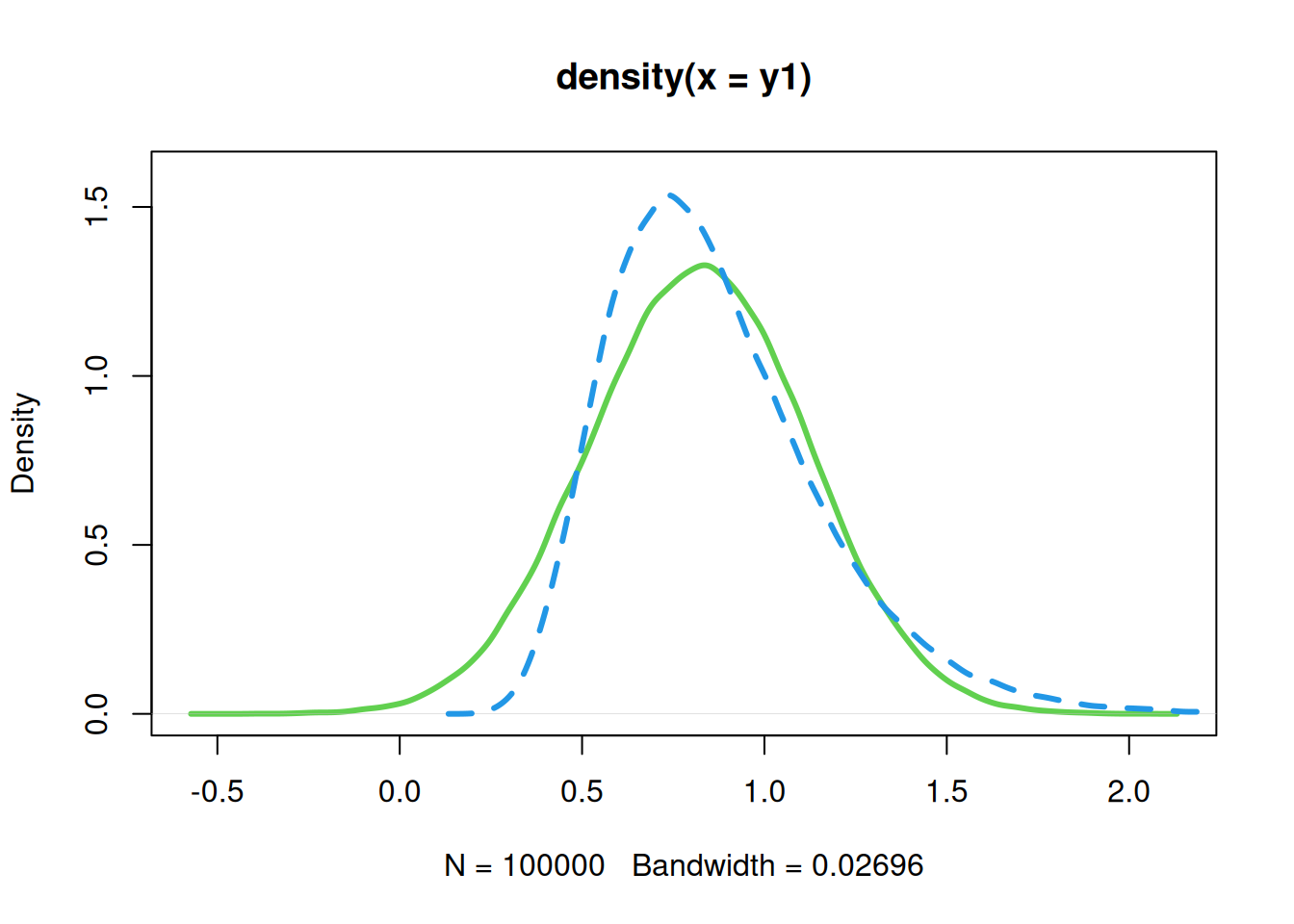
gsd
mu <- 1.48
sig <- 0.074
(sdlog <- find_lognormal_sd(mu, sig))
#> [1] 0.04990982
y1 <- rnorm(n = Nsim, mean = mu, sd = sig)
y2 <- exp(rnorm(n = Nsim, log(mu), sdlog))
summary(y1)
#>    Min. 1st Qu.  Median    Mean 3rd Qu.    Max.
#>   1.188   1.429   1.479   1.479   1.529   1.817
summary(y2)
#>    Min. 1st Qu.  Median    Mean 3rd Qu.    Max.
#>   1.212   1.431   1.480   1.482   1.530   1.825
plot(density(y1), col = 3, lwd = 3, ylim = c(0, 6))
lines(density(y2), col = 4, lwd = 3, lty = 2)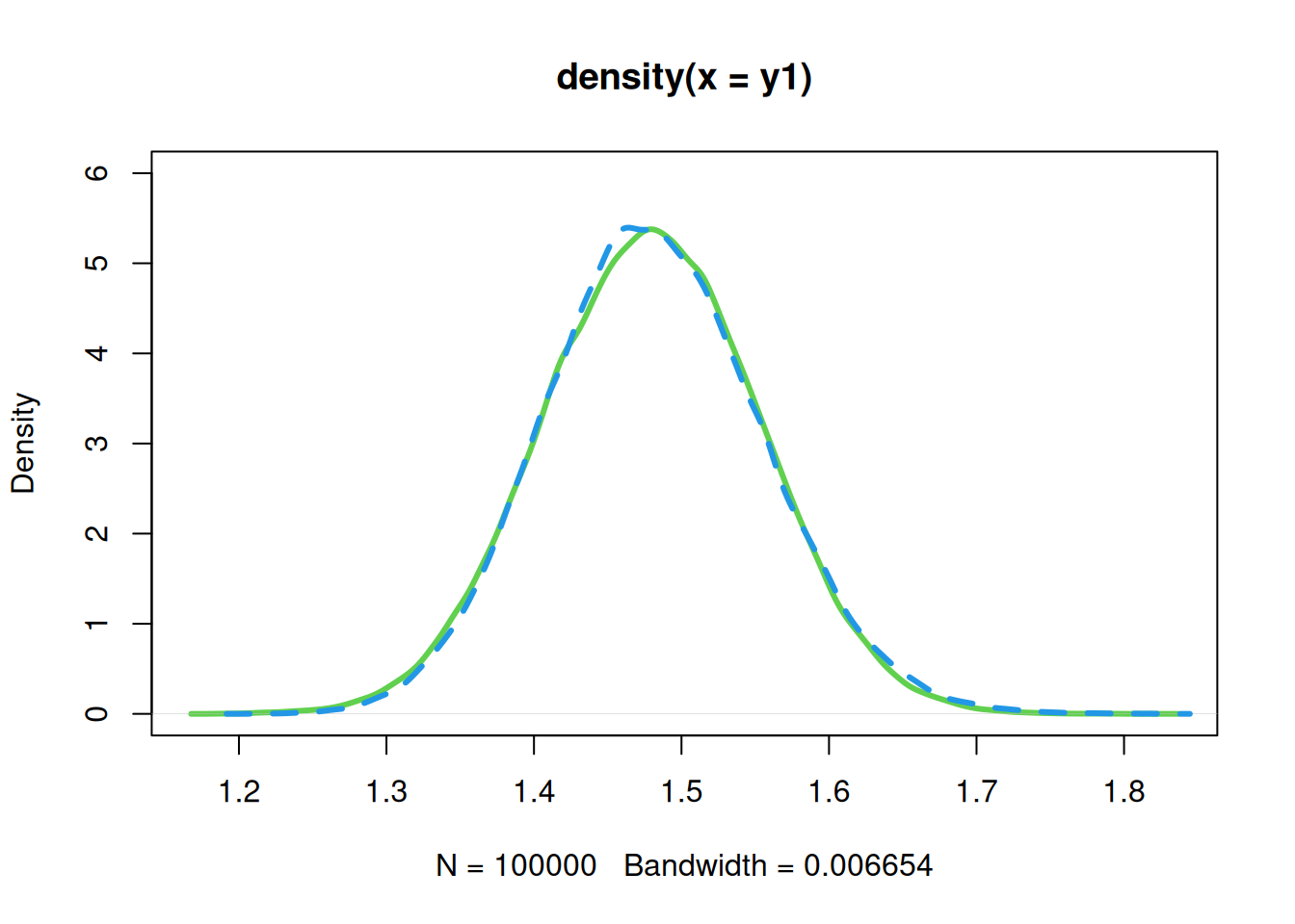
sel50
Selectivity parameters are given weakly informative priors centred on the minimum legal size for the fishery (Punt et al. 2013).
mu <- 50
sig <- 30
(sdlog <- find_lognormal_sd(mu, sig))
#> [1] 0.4976548
y1 <- rnorm(n = Nsim, mean = mu, sd = sig)
y2 <- exp(rnorm(n = Nsim, log(mu), sdlog))
summary(y1)
#>    Min. 1st Qu.  Median    Mean 3rd Qu.    Max.
#>  -69.58   29.75   50.01   50.00   70.35  174.96
summary(y2)
#>    Min. 1st Qu.  Median    Mean 3rd Qu.    Max.
#>   6.008  35.780  50.060  56.747  70.103 428.579
plot(density(y1), col = 3, lwd = 3, ylim = c(0, 0.02))
lines(density(y2), col = 4, lwd = 3, lty = 2)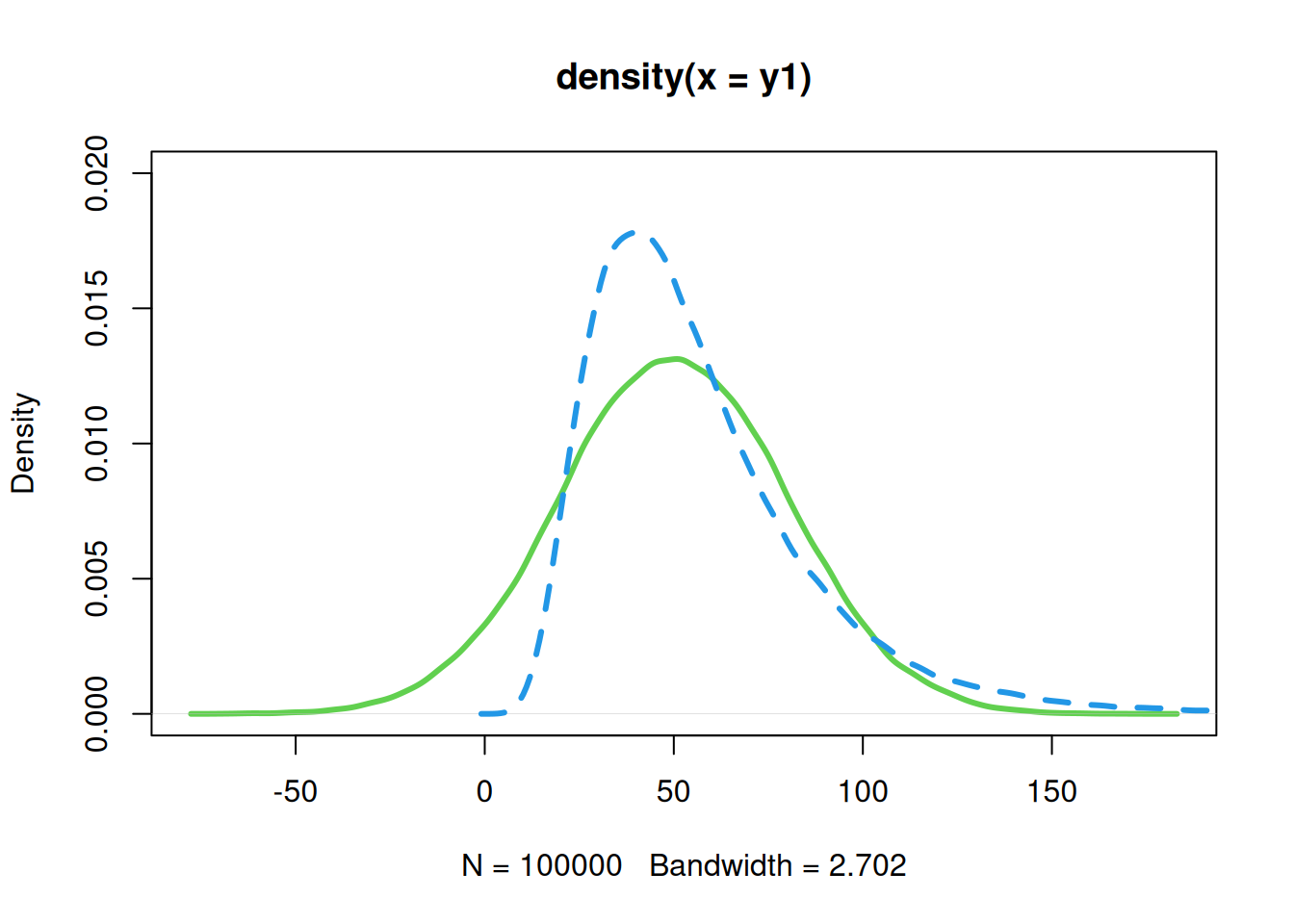
sel95
mu <- 10
sig <- 30
(sdlog <- find_lognormal_sd(mu, sig))
#> [1] 1.124519
y1 <- rnorm(n = Nsim, mean = mu, sd = sig)
y2 <- exp(rnorm(n = Nsim, log(mu), sdlog))
summary(y1)
#>    Min. 1st Qu.  Median    Mean 3rd Qu.    Max.
#> -124.32  -10.25   10.00   10.02   30.22  135.41
summary(y2)
#>      Min.   1st Qu.    Median      Mean   3rd Qu.      Max.
#> 6.475e-02 4.678e+00 9.976e+00 1.875e+01 2.129e+01 1.027e+03
plot(density(y1), col = 3, lwd = 3, ylim = c(0, 0.2))
lines(density(y2), col = 4, lwd = 3, lty = 2)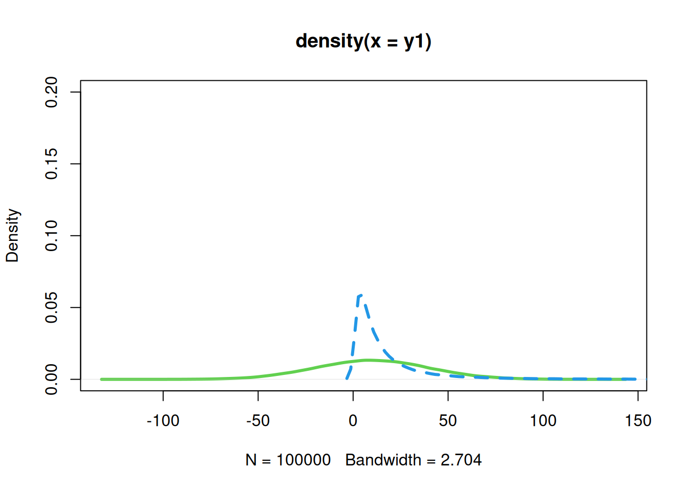
selmax
Maximum vulnerability is positive. Moment matching a log-Normal prior to a natural-scale mean of 1 and standard deviation of 1 gives .
Rmu, Rsd, Rsigma
hist(exp(rnorm(Nsim, log(32), 0.1)))
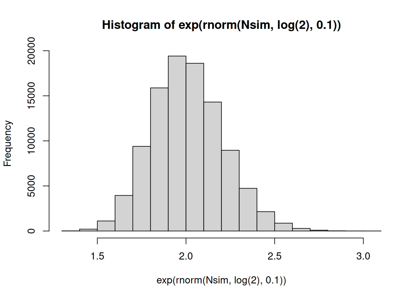
hist(exp(rnorm(Nsim, log(2), 0.1)))
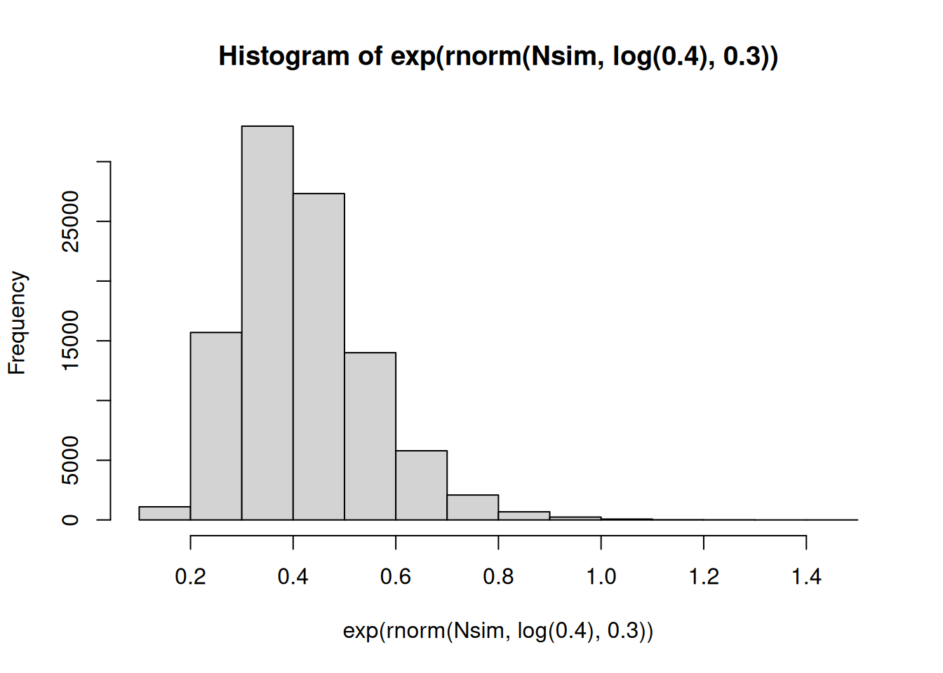
hist(exp(rnorm(Nsim, log(0.4), 0.3)))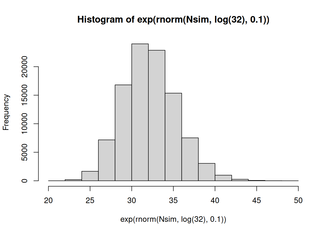
Clark, William G. 1999. “Effects of an Erroneous Natural Mortality Rate on a Simple Age-Structured Stock Assessment.” Canadian Journal of Fisheries and Aquatic Sciences 56 (10): 1721–31. https://doi.org/10.1139/f99-085.
Hilborn, Ray, and Carl J. Walters. 1992. Quantitative Fisheries Stock Assessment: Choice, Dynamics and Uncertainty. Chapman; Hall. https://doi.org/10.1007/978-1-4615-3598-0.
Kristensen, Kasper, Anders Nielsen, Casper W. Berg, Hans Skaug, and Bradley M. Bell. 2016. “TMB: Automatic Differentiation and Laplace Approximation.” Journal of Statistical Software 70 (5): 1–21. https://doi.org/10.18637/jss.v070.i05.
Punt, André E., Tao-Cheng Huang, and Mark N. Maunder. 2013. “Review of Integrated Size-Structured Models for Stock Assessment of Hard-to-Age Crustacean and Mollusc Species.” ICES Journal of Marine Science 70 (1): 16–33. https://doi.org/10.1093/icesjms/fss185.
Quinn, Terrance J., and Richard B. Deriso. 1999. Quantitative Fish Dynamics. Oxford University Press.