
# remotes::install_github("noaa-afsc/SparseNUTS")
if (dir.exists(file.path("..", "R")) && requireNamespace("pkgload", quietly = TRUE)) {
  pkgload::load_all("..", quiet = TRUE)
} else {
  library(decamod)
}
library(TMBhelper)
library(tidyverse)
library(kableExtra)
library(SparseNUTS)

theme_set(theme_bw())

options(mc.cores = parallel::detectCores() - 1) # Specify the number of cores

tags <- tags_all %>%
  filter(RelStatArea %in% 905:908) %>% # CRA 2
  # filter(RelStatArea %in% c(939, 934, 927:928, 929:931, 935:938)) %>%
  rename(gi_L1 = RelLngth, gi_L2 = RecLngth) %>%
  mutate(gi_obs = gi_L2 - gi_L1) %>%
  mutate(gi_liberty = DaysatLiberty / 365) %>%
  mutate(gi_sex = as.integer(Sex)) %>%
  filter(gi_liberty > 0.5, gi_obs > -10) %>%
select(gi_sex, gi_L1, gi_liberty, gi_obs)Load inputs
This vignette uses CRA 2 tag-recapture data (statistical areas 905–908). Tag-recapture data are collected from rock lobster fisheries and used to estimate growth parameters (Webber and Stephenson 2016; Schnute and Fournier 1980).
Define model
The Schnute–Francis reference-increment model (Schnute and Fournier 1980) is fitted to tag-recapture data to estimate size-based growth increments. Below, it is compared with the corresponding constrained generalized coordinates and with the selected monotone-ODE structure. The remainder of the vignette deliberately continues with the Schnute–Francis fit so that the established diagnostic examples are unchanged.
data <- list(
  growth_model = 1, # 1=Schnute-Francis, 2=generalized Linf/K/gamma
  growth_like = 3, # 0=off, 1=normal, 2=robust-normal, 3=student-t
  growth_df = 3, # Student-t degrees of freedom; must be greater than 2
  n_growth = 2, # males and females
  n_sex = 2,
  l_sex = c("Male", "Female"),
  ga = 50, gb = 80, gmin = 0,
  # Used only for growth_model = 2 with prior_on = 1. These are priors on
  # sampled log(Linf), log(K), and log(gamma), so no Jacobian is needed.
  log_linf_prior_mean = log(rep(120, 2)),
  log_linf_prior_sd = rep(0.5, 2),
  log_k_prior_mean = log(rep(0.1, 2)),
  log_k_prior_sd = rep(0.7, 2),
  log_gshape_prior_mean = log(rep(2, 2)),
  log_gshape_prior_sd = rep(0.6, 2),
  jacobian_on = 0, prior_on = 0, like_on = 1)
data <- c(data, as.list(tags))
Define the parameters list. Create the AD object using the MakeADFun function.
parameters <- list(
  log_linf = log(c(100, 100)),
  log_k = log(c(0.1, 0.1)),
  log_galpha = log(c(6.837, 4.978)),
  logit_gdiff = qlogis(c(2.439/6.837, 1.149/4.978)),
  log_gshape = log(c(2.4, 4.037)),
  log_gcv = log(c(0.4366, 0.7335)),
  log_gobs = log(2.5)
)

if (data$growth_model == 1) {
  map <- list(
    log_linf = factor(rep(NA, length(parameters$log_linf))),
    log_k = factor(rep(NA, length(parameters$log_k)))
  )
} else {
  map <- list(
    log_galpha = factor(rep(NA, length(parameters$log_galpha))),
    logit_gdiff = factor(rep(NA, length(parameters$logit_gdiff)))
  )
}

obj <- MakeADFun(func = cmb(growth_model, data), parameters = parameters, map = map)
Define parameter bounds.
Lwr <- rep(-Inf, length(obj$par))
Upr <- rep(Inf, length(obj$par))

Lwr[grep("log_linf", names(obj$par))] <- log(max(data$gi_L1) + 1)
Upr[grep("log_linf", names(obj$par))] <- log(200)
Lwr[grep("log_k", names(obj$par))] <- log(0)
Upr[grep("log_k", names(obj$par))] <- log(1)
Lwr[grep("log_galpha", names(obj$par))] <- log(0)
Upr[grep("log_galpha", names(obj$par))] <- log(20)
# Lwr[grep("logit_gdiff", names(obj$par))] <- qlogis(0.001)
# Upr[grep("logit_gdiff", names(obj$par))] <- qlogis(0.999)
Lwr[grep("log_gshape", names(obj$par))] <- log(0.1)
Upr[grep("log_gshape", names(obj$par))] <- log(15)
Lwr[grep("log_gcv", names(obj$par))] <- log(0.01)
Upr[grep("log_gcv", names(obj$par))] <- log(2)
Lwr[grep("log_gobs", names(obj$par))] <- log(0.00001)
Upr[grep("log_gobs", names(obj$par))] <- log(10)

tibble(Parameter = names(obj$par), LB = Lwr, Initial = obj$par, UB = Upr)
#> # A tibble: 9 × 4
#>   Parameter        LB Initial      UB
#>   <chr>         <dbl>   <dbl>   <dbl>
#> 1 log_galpha  -Inf      1.92    3.00
#> 2 log_galpha  -Inf      1.61    3.00
#> 3 logit_gdiff -Inf     -0.590 Inf
#> 4 logit_gdiff -Inf     -1.20  Inf
#> 5 log_gshape    -2.30   0.875   2.71
#> 6 log_gshape    -2.30   1.40    2.71
#> 7 log_gcv       -4.61  -0.829   0.693
#> 8 log_gcv       -4.61  -0.310   0.693
#> 9 log_gobs     -11.5    0.916   2.30
Optimise using the nlminb function:
control <- list(eval.max = 100000, iter.max = 100000)
opt <- nlminb(start = obj$par, objective = obj$fn, gradient = obj$gr,
              control = control, lower = Lwr, upper = Upr)
opt <- nlminb(start = opt$par, objective = obj$fn, gradient = obj$gr,
              control = control, lower = Lwr, upper = Upr)
obj$par <- opt$par
obj$env$last.par <- opt$par
obj$env$last.par.best <- opt$par
exp(opt$par[names(opt$par) %in% c("log_gcv", "log_gobs")])
tibble(par = names(obj$par), val = obj$par, gr = obj$gr()[1,]) %>% arrange(-gr)
#> outer mgc:  0.005112041
#> # A tibble: 9 × 3
#>   par            val          gr
#>   <chr>        <dbl>       <dbl>
#> 1 log_galpha   1.98   0.00511
#> 2 log_galpha   1.96   0.00175
#> 3 logit_gdiff -2.11   0.000431
#> 4 log_gcv     -0.685  0.000269
#> 5 log_gcv     -0.271  0.00000753
#> 6 logit_gdiff -1.44  -0.000118
#> 7 log_gobs     1.07  -0.000166
#> 8 log_gshape   1.18  -0.000206
#> 9 log_gshape   2.04  -0.00110
# check_estimability(obj = obj)
obj$simulate(par = obj$env$last.par.best)$gi_obs[1:10]
#>  [1]  9.8934460  5.0207657  4.0035990  4.4509891  5.4566757  5.8389251
#>  [7]  2.6758796 -0.8660002 10.3657378  1.0502963
# osa <- oneStepPredict(obj = obj, observation.name = "gi_obs", method = "oneStepGeneric", trace = FALSE)
# qqnorm(osa$res); abline(0, 1)
# osa2 <- oneStepPredict(obj = obj, method = "fullGaussian", discrete = FALSE, trace = FALSE)
# qqnorm(osa2$res); abline(0, 1)
# plot(data$gi_L1, osa$residual)
# plot(data$gi_liberty, osa$residual)
# plot(data$gi_obs, osa$residual)
# chk <- checkConsistency(obj = obj, hessian = TRUE, estimate = TRUE, n = 200)
# chk
# s <- summary(chk)
# s
# s$marginal$p.value
breaks <- c(seq(30, 90, 2), Inf)
bins <- cut(x = seq(31, 91, 2), breaks = breaks, right = FALSE)
midpoint_l <- midcut(x = seq(31, 91, 2), from = 30, to = 92, by = 2)

length(breaks)
#> [1] 32
length(bins)
#> [1] 31
length(midpoint_l)
#> [1] 31

tibble(bins, midpoint_l) %>% head(3)
#> # A tibble: 3 × 2
#>   bins    midpoint_l
#>   <fct>        <dbl>
#> 1 [30,32)         31
#> 2 [32,34)         33
#> 3 [34,36)         35
tibble(bins, midpoint_l) %>% tail(3)
#> # A tibble: 3 × 2
#>   bins     midpoint_l
#>   <fct>         <dbl>
#> 1 [86,88)          87
#> 2 [88,90)          89
#> 3 [90,Inf)         91

tibble(test = c(27, 30, 30.1, 31, 31.9, 32, 90, 91, 150)) %>%
  mutate(bin = cut(x = test, breaks = breaks, right = FALSE))
#> # A tibble: 9 × 2
#>    test bin
#>   <dbl> <fct>
#> 1  27   <NA>
#> 2  30   [30,32)
#> 3  30.1 [30,32)
#> 4  31   [30,32)
#> 5  31.9 [30,32)
#> 6  32   [32,34)
#> 7  90   [90,Inf)
#> 8  91   [90,Inf)
#> 9 150   [90,Inf)

l_sex <- c("Male", "Female") # plot labels
plot_growth_increment(data = data, parameters = parameters, obj = obj, tau = 1,
                      midpoint = midpoint_l)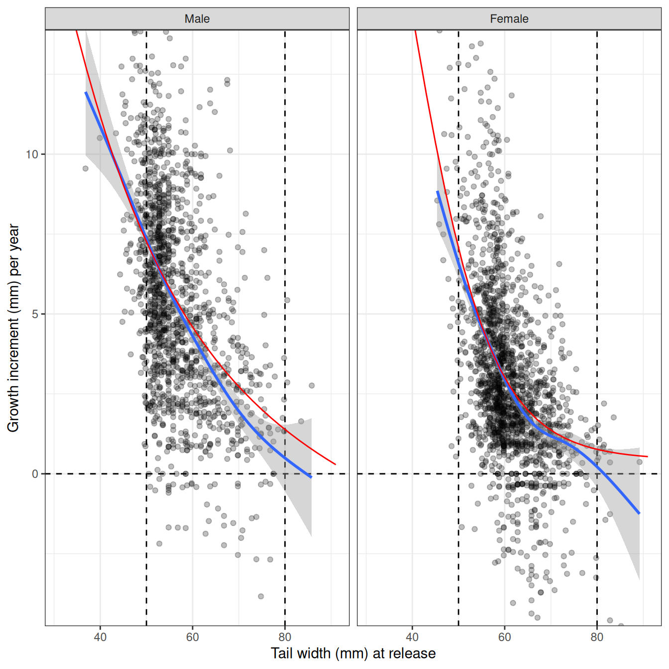
Three growth-curve options
The first two options below are fitted to the same CRA 2 tags and likelihood. The generalized option uses the same deterministic Schnute growth equation but restricts it to a positive finite asymptote, positive rate, and bounded shape. It is therefore an exact reparameterization only when the fitted reference-increment coordinates imply a valid pair; the CRA 2 female Schnute–Francis optimum does not, so that line also illustrates the effect of the new constraints. The ODE line uses the CRA 2 coordinates from the selected support-gated all-QMA fit. It is evaluated here, rather than fitted to these tags again, because its role in an assessment is as an externally conditioned growth curve or an external multivariate prior.
schnute_parameters <- obj$env$parList(obj$env$last.par.best)
schnute_as_linf <- growth_francis_to_linf(
  ga = data$ga,
  gb = data$gb,
  galpha = exp(schnute_parameters$log_galpha),
  gbeta = plogis(schnute_parameters$logit_gdiff) *
    exp(schnute_parameters$log_galpha),
  gshape = exp(schnute_parameters$log_gshape)
)
generalized_data <- data
generalized_data$growth_model <- 2L
generalized_parameters <- schnute_parameters
generalized_initial_linf <- ifelse(
  schnute_as_linf$valid,
  schnute_as_linf$linf,
  max(data$gi_L1) + 15
)
generalized_initial_k <- ifelse(
  schnute_as_linf$valid,
  schnute_as_linf$k,
  0.03
)
generalized_parameters$log_linf <- log(generalized_initial_linf)
generalized_parameters$log_k <- log(generalized_initial_k)
generalized_map <- list(
  log_galpha = factor(rep(NA, data$n_growth)),
  logit_gdiff = factor(rep(NA, data$n_growth))
)
generalized_obj <- MakeADFun(
  func = cmb(growth_model, generalized_data),
  parameters = generalized_parameters,
  map = generalized_map,
  silent = TRUE
)
generalized_lower <- rep(-Inf, length(generalized_obj$par))
generalized_upper <- rep(Inf, length(generalized_obj$par))
generalized_lower[grepl("^log_linf$", names(generalized_obj$par))] <-
  log(max(data$gi_L1) + 1)
generalized_upper[grepl("^log_linf$", names(generalized_obj$par))] <- log(200)
generalized_lower[grepl("^log_k$", names(generalized_obj$par))] <- log(1e-4)
generalized_upper[grepl("^log_k$", names(generalized_obj$par))] <- log(2)
generalized_lower[grepl("^log_gshape$", names(generalized_obj$par))] <- log(1)
generalized_upper[grepl("^log_gshape$", names(generalized_obj$par))] <- log(8)
generalized_lower[grepl("^log_gcv$", names(generalized_obj$par))] <- log(0.01)
generalized_upper[grepl("^log_gcv$", names(generalized_obj$par))] <- log(2)
generalized_lower[grepl("^log_gobs$", names(generalized_obj$par))] <- log(1e-5)
generalized_upper[grepl("^log_gobs$", names(generalized_obj$par))] <- log(10)
generalized_opt <- nlminb(
  generalized_obj$par,
  generalized_obj$fn,
  generalized_obj$gr,
  lower = generalized_lower,
  upper = generalized_upper,
  control = control
)
generalized_opt <- nlminb(
  generalized_opt$par,
  generalized_obj$fn,
  generalized_obj$gr,
  lower = generalized_lower,
  upper = generalized_upper,
  control = control
)
generalized_gradient <- as.numeric(
  generalized_obj$gr(generalized_opt$par)
)
generalized_projected_gradient <- generalized_gradient
generalized_projected_gradient[
  generalized_opt$par <= generalized_lower + 1e-8 &
    generalized_projected_gradient > 0
] <- 0
generalized_projected_gradient[
  generalized_opt$par >= generalized_upper - 1e-8 &
    generalized_projected_gradient < 0
] <- 0
stopifnot(
  generalized_opt$convergence == 0,
  max(abs(generalized_projected_gradient)) < 0.01
)
generalized_obj$par <- generalized_opt$par
generalized_obj$env$last.par <- generalized_opt$par
generalized_obj$env$last.par.best <- generalized_opt$par

# CRA 2 coordinates from the selected support-gated all-QMA monotone-ODE fit.
cra2_ode_coordinate <- c(
  -1.367895, 0.138464, 2.803002, 0.682680, 0.681610,
  -0.094374, 1.387688, 4.114626, 0.604917, 0.755512,
  2.202328, -0.399832, 0, 1.331421,
  2.121850, -0.466410, 0, 1.192002,
  -0.635750
)
comparison_length <- seq(30, 90, by = 0.5)
generalized_report <- generalized_obj$report(
  generalized_obj$env$last.par.best
)

growth_option_curves <- map_dfr(seq_len(data$n_growth), function(group) {
  schnute_curve <- get_growth_increment(
    midpoint = comparison_length,
    ga = data$ga,
    gb = data$gb,
    galpha = exp(schnute_parameters$log_galpha[group]),
    gbeta = plogis(schnute_parameters$logit_gdiff[group]) *
      exp(schnute_parameters$log_galpha[group]),
    gshape = exp(schnute_parameters$log_gshape[group]),
    gcv = exp(schnute_parameters$log_gcv[group]),
    gobs = NULL,
    gdd = 0,
    gmin = data$gmin,
    biomass = 1,
    tau = 1
  )$gi
  generalized_curve <- get_growth_increment_linf(
    midpoint = comparison_length,
    linf = generalized_report$linf[group],
    k = generalized_report$growth_rate[group],
    gshape = generalized_report$gshape[group],
    gcv = exp(generalized_obj$env$parList(
      generalized_obj$env$last.par.best
    )$log_gcv[group]),
    gobs = NULL,
    gmin = data$gmin,
    tau = 1
  )$gi
  ode_curve <- get_growth_increment_ode(
    midpoint = comparison_length,
    tau = 1,
    growth_group = group,
    growth_ode_coordinate = cra2_ode_coordinate
  )$gi
  tibble(
    Sex = data$l_sex[group],
    `Release length` = rep(comparison_length, 3),
    `Annual increment` = c(schnute_curve, generalized_curve, ode_curve),
    Model = factor(
      rep(c(
        "Schnute–Francis reference increments",
        "Generalized Linf/K/gamma",
        "Selected monotone ODE"
      ), each = length(comparison_length)),
      levels = c(
        "Schnute–Francis reference increments",
        "Generalized Linf/K/gamma",
        "Selected monotone ODE"
      )
    )
  )
})

ggplot(
  growth_option_curves,
  aes(`Release length`, `Annual increment`, colour = Model, linetype = Model)
) +
  geom_line(linewidth = 0.9) +
  facet_wrap(~ Sex) +
  scale_y_continuous(
    limits = c(0, NA),
    expand = expansion(mult = c(0, 0.04))
  ) +
  labs(
    x = "Release tail width (mm)",
    y = "Annual increment (mm)",
    colour = NULL,
    linetype = NULL
  ) +
  theme(legend.position = "bottom")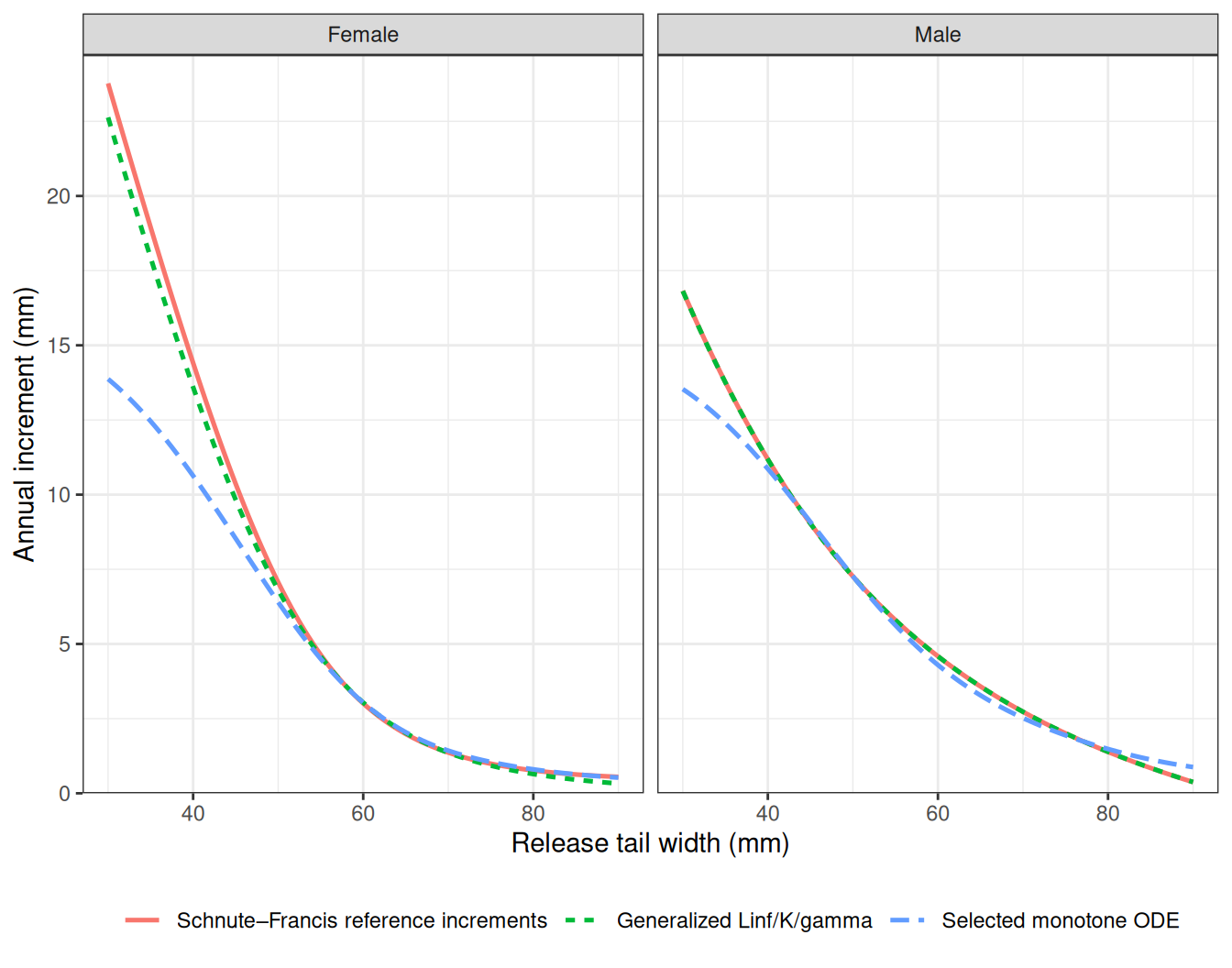
plot_growth_density(data = data, obj = obj, nsim = 100, type = 1) +
  coord_cartesian(xlim = c(-15, 25))
# plot_growth_density(data = data, obj = obj, report = obj$report(obj$env$last.par.best),
#                     simulate = obj$simulate(par = obj$env$last.par.best), nsim = 50, type = 1)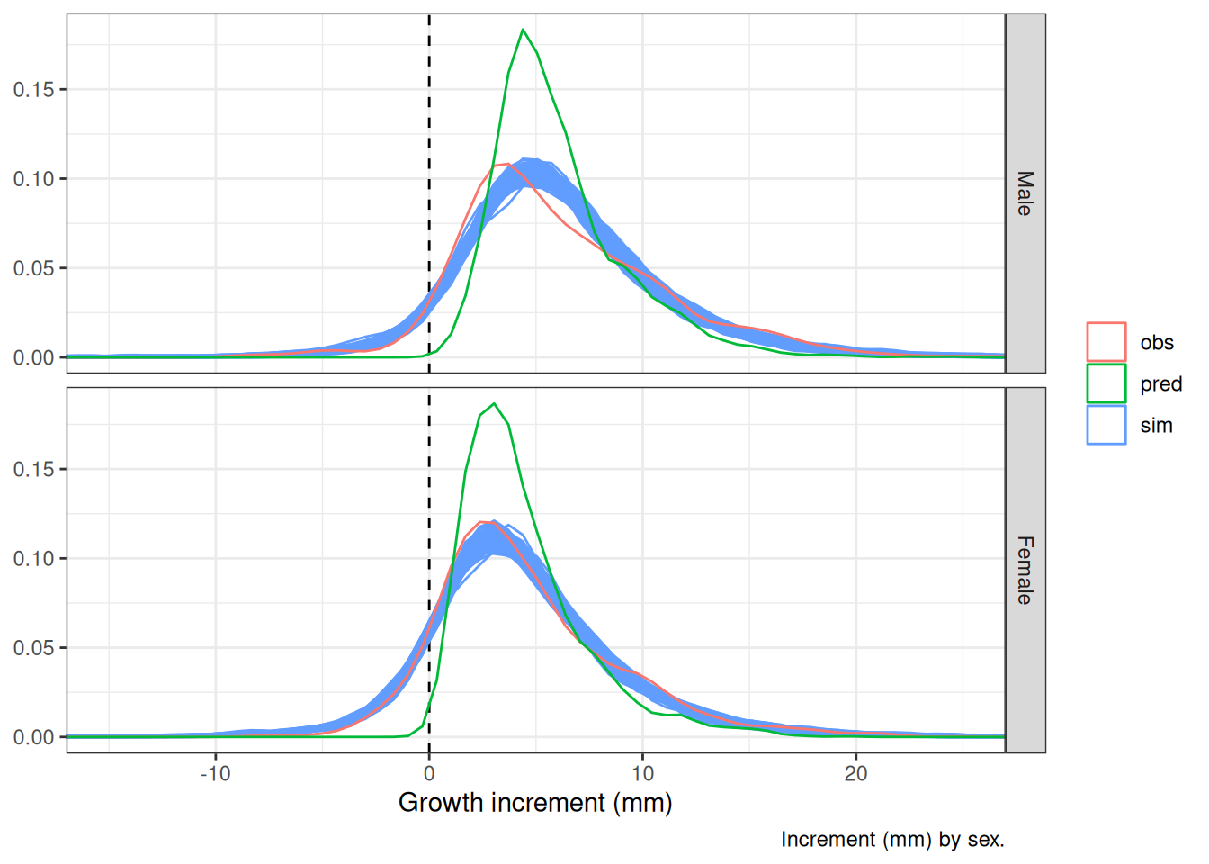
plot_growth_density(data = data, obj = obj, nsim = 100, type = 2) +
  coord_cartesian(xlim = c(-15, 25))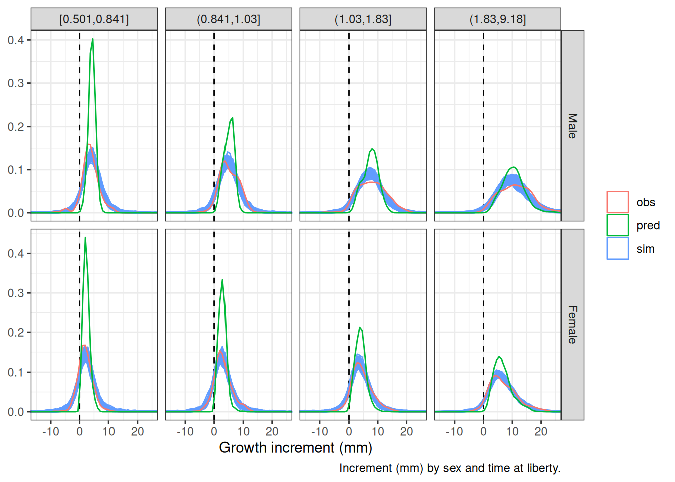
plot_growth_density(data = data, obj = obj, nsim = 100, type = 3) +
  coord_cartesian(xlim = c(-15, 25))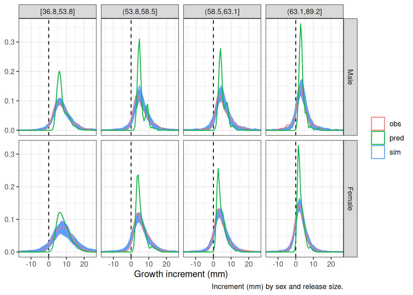
Bayesian inference
Bayesian inference is performed using the NUTS sampler via automatic differentiation (Kristensen et al. 2016). The priors in this model are defined directly on the sampled log and logit parameters, so no transformation Jacobian is required and jacobian_on remains zero:
# data$jacobian_on <- 0
# data$like_on <- 1
# data$prior_on <- 1
# obj <- MakeADFun(func = cmb(growth_model, data), parameters = parameters)
# obj$par <- opt$par
Using Cole Monnahan’s adnuts package, we can run the MCMC sampler. The adnuts package is a wrapper around the NUTS sampler in Stan.
# mcmc <- sample_sparse_tmb(
#   obj = obj, metric = "auto", iter = 4000, warmup = 3000, chains = 4, cores = 4,
#   control = list(adapt_delta = 0.99), init = "last.par.best", globals = decamod_globals())
# mcmc1 <- sample_snuts(
#   obj = obj, metric = "auto", num_samples = 1000, chains = 4, cores = 4,
#   control = list(adapt_delta = 0.99), init = "last.par.best",
#   # lower = Lwr, upper = Upr,
#   globals = list(get_growth_increment = get_growth_increment,
#                  get_growth_increment_vb = get_growth_increment_vb,
#                  drobust = drobust, dstudent_t_sd = dstudent_t_sd,
#                  jac_exp = jac_exp, jac_invlogit = jac_invlogit))
# library(priorsense)
# lp <- get_posterior(object = obj, posterior = mcmc1, pars = c("loglikes", "priors"), type = "array")
# samps <- extract_samples(fit = mcmc1, inc_lp = FALSE, as.list = FALSE)
# samps$lprior <- as.numeric(lp$priors[,,1])
# samps$log_lik <- as.numeric(lp$loglikes[,,1])
# psd <- create_priorsense_data(x = samps)
# powerscale_sensitivity(psd)
# powerscale_plot_dens(psd, variable = "log_galpha")
# powerscale_plot_ecdf(psd)
# powerscale_plot_quantities(psd)
#
# x <- example_powerscale_model()
# psd <- create_priorsense_data(x$draws)
# powerscale_sensitivity(psd)
# powerscale_plot_dens(psd)
# powerscale_plot_ecdf(psd)
# powerscale_plot_quantities(psd)
# plot_sampler_params(fit = mcmc1, plot = TRUE)
# pairs_rtmb(fit = mcmc1, order = "mismatch", pars = 1:5)
# pairs_rtmb(fit = mcmc1, order = "slow", pars = 1:5)
# pairs_rtmb(fit = mcmc1, order = "fast", pars = 1:5)
# plot_marginals(fit = mcmc1)
# plot_uncertainties(fit = mcmc1, log = TRUE, plot = TRUE)
plot_priors <- function(nsim = 100000) {
  nsim <- 100000

  df_posterior <-  reshape2::melt(mcmc1$samples) %>%
    rename(variable = Var3) %>%
    filter(variable != "lp__") %>%
    mutate(value = ifelse(grepl("logit_", variable), plogis(value), exp(value))) %>%
    mutate(variable = gsub("log_", "", variable)) %>%
    mutate(variable = gsub("logit_", "", variable))

  head(df_posterior)

  df_priors <- tibble(
    "galpha[1]" = exp(rnorm(nsim, log(3), 0.5)),
    "galpha[2]" = exp(rnorm(nsim, log(3), 0.5)),
    "gdiff[1]" = plogis(rnorm(nsim, -1, 1.5)),
    "gdiff[2]" = plogis(rnorm(nsim, -1, 1.5)),
    "gshape[1]" = exp(rnorm(nsim, log(4.81), 0.4)),
    "gshape[2]" = exp(rnorm(nsim, log(4.51), 0.4)),
    "gcv[1]" = exp(rnorm(nsim, log(0.59), 0.4)),
    "gcv[2]" = exp(rnorm(nsim, log(0.82), 0.4)),
    "gobs" = exp(rnorm(nsim, log(1.48), 0.3))) %>%
    reshape2::melt()

  head(df_priors)

  ggplot(data = df_priors, aes(x = value)) +
    # geom_density(fill = "red", color = NA, alpha = 0.5) +
    geom_histogram(aes(y = after_stat(density)), fill = "red", color = NA, alpha = 0.5) +
    geom_histogram(data = df_posterior, aes(y = after_stat(density)), fill = "blue", color = NA, alpha = 0.5) +
    facet_wrap(variable ~ ., scales = "free")
}
# library(posterior)
# mc <- mcmc1$samples %>% as_draws_df() %>%
#   subset_draws(iteration = 1001:2000)
# #   rename_variables(galpha = log_galpha, gbeta = log_gbeta, gshape = log_gshape) %>%
# #   mutate_variables(gobs = exp(log_gobs))
# #   # merge_chains()
# summarise_draws(mc)
# mc
# variables(mc)
# # summarise_draws(mc, ~exp(.x))
# # summarise_draws(mc, ~quantile(.x, probs = c(0.4, 0.6)))
#
# # obj$par <- summarise_draws(mc)$median[1:9]
#
# # np <- mcmc1@diagnostics %>%
# #   as_draws_matrix() %>%
# #   as_draws_array()
# # nuts_params(mcmc1@diagnostics)
#
# library(bayesplot)
# mcmc_areas(x = mc, #transformations = "exp",
#            regex_pars = c("log_galpha", "log_gbeta", "log_gshape", "log_gcv", "log_gobs"))
# # np <- nuts_params(mc)
# # mcmc_trace(mc, np = np)
# # mcmc_trace(mc, transformations = list("log_galpha[1]" = "exp"))
# # mcmc_trace(mc, regex_pars = c("log_galpha", "log_gbeta", "log_gshape", "log_gcv", "log_gobs"), transformations = "exp")
# mcmc_trace_highlight(mc)
# mcmc_rank_ecdf(mc)
# mcmc_rank_hist(mc)
# library(StanEstimators)
# library(posterior)
# mcmc1 <- stan_sample(fn = function(x) -obj$fn(x),
#                      grad_fun = function(x) -obj$gr(x),
#                      par_inits = opt$par, lower = Lwr, upper = Upr,
#                      num_chains = 4, parallel_chains = 4, seed = 42,
#                      packages = c("RTMB", "decamod"))
# # check_hmc_diagnostics(object = mcmc1)
# class(mcmc1)
# summary(mcmc1)
#
# posterior <- unconstrain_draws(mcmc1) %>%
#   as_draws_matrix()
# variables(posterior) <- c("lp__", make.unique(names(obj$par)))
# posterior
# variables(posterior)
#
# # np <- mcmc1@diagnostics %>%
# #   as_draws_matrix() %>%
# #   as_draws_array()
# # nuts_params(mcmc1@diagnostics)
#
# library(bayesplot)
#
# mcmc_areas(x = posterior, #transformations = "exp",
#            pars = c("log_galpha", "log_galpha.1", "log_gbeta", "log_gbeta.1", "log_gshape", "log_gshape.1", "log_gcv", "log_gcv.1", "log_gobs"),
#            prob = 0.8)
#
# # mcmc_trace(posterior, np = np)
# mcmc_trace(posterior, transformations = "exp")
Can I recover priors:
# https://github.com/kaskr/tmbstan
# devtools::install_github("kaskr/tmbstan/tmbstan")
# library(tmbstan)
# # Needed for more than 1 chain
# init_fn <- function() {
#   list(log_galpha = runif(2, 1.5, 1.7), log_gbeta = runif(2, 0.6, 0.7),
#        log_gshape = runif(2, 1, 1.5),
#        log_gcv = runif(2, -0.7, -0.5), log_gobs = runif(1, 0, 0.1))
# }
#
# n_chains <- 1
# # Broken
# mcmc2 <- tmbstan(obj = obj,
#                  # init = init_fn,
#                  # init = rep(list(parameters), n_chains),
#                  init = "last.par.best", iter = 10000, warmup = 5000,
#                  # open_progress = FALSE,
#                  # lower = Lwr, upper = Upr,
#                  chains = 1)
#                  # control = list(max_treedepth = 12, adapt_delta = 0.9))

# data2 <- data
# data2$jacobian_on <- 0
# data2$prior_on <- 1
# data2$like_on <- 0
# obj2 <- MakeADFun(func = cmb(growth_model, data2), parameters = parameters)
# obj2$par <- opt$par
# tibble(Parameter = names(obj$par), LB = Lwr, Initial = obj$par, UB = Upr)
# library(StanEstimators)
# mcmc2 <- stan_sample(fn = function(x) -obj2$fn(x),
#                      grad_fun = function(x) -obj2$gr(x),
#                      par_inits = c(2, 2, 0, 0, 1, 1, 0, 0, 0),
#                      lower = Lwr, upper = Upr,
#                      num_chains = 1,
#                      # num_chains = 4, parallel_chains = 4, seed = 42,
#                      packages = c("RTMB", "decamod"))
#
# library(bayesplot)
# names(mcmc2@draws) <- c("lp__", "log_galpha1", "log_galpha2", "logit_gdiff1", "logit_gdiff2",
#                         "log_gshape1", "log_gshape2", "log_gcv1", "log_gcv2",
#                         "log_gobs", ".chain", ".iteration", ".draw")
# mcmc_trace(mcmc2@draws)

# df <- reshape2::melt(mcmc2@draws) %>% filter(variable == "logit_gdiff1")
# hist(df$value)
# hist(plogis(df$value))
# range(df$value)
# df$value[df$value > 1]
# plogis(-709)
# plogis(36)

# df <- reshape2::melt(mcmc2@draws) %>%
#   filter(!(variable %in% c("lp__", ".chain", ".iteration", ".draw"))) %>%
#   # mutate(value = ifelse(grepl("log_", variable), exp(value), plogis(value))) %>%
#   mutate(value = ifelse(grepl("logit_", variable), plogis(value), exp(value))) %>%
#   mutate(variable = gsub("log_", "", variable)) %>%
#   mutate(variable = gsub("logit_", "", variable))
# tail(df)
#
# nsim <- 4000
# df_priors <- data.frame(galpha1 = rnorm(nsim, 2, 30), galpha2 = rnorm(nsim, 2, 30),
#                         gdiff1 = rbeta(nsim, 1, 1), gdiff2 = rbeta(nsim, 1, 1),
#                         gshape1 = rnorm(nsim, 4.81, 1), gshape2 = rnorm(nsim, 4.51, 1),
#                         gcv1 = rnorm(nsim, 0.59, 0.3), gcv2 = rnorm(nsim, 0.82, 0.3),
#                         gobs = rnorm(nsim, 1.48, 0.074)) %>% reshape2::melt()
#
# ggplot(data = df) +
#   geom_histogram(aes(x = value)) +
#   geom_histogram(data = df_priors, aes(x = value), fill = "red", color = NA, alpha = 0.5) +
#   facet_wrap(variable ~ ., scales = "free")
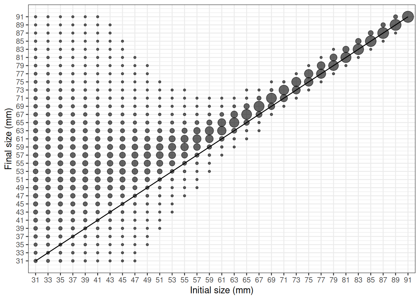
Growth matrix
The growth transition matrix describes the probability of an individual moving from one length class to another over a given time period (Quinn and Deriso 1999; Hilborn and Walters 1992).
plot_growth_matrix <- function() {
  par(mfrow = c(1, 2))
  for (isex in 1:2) {
    increment <- get_growth_increment(
      midpoint = midpoint_l, ga = data$ga, gb = data$gb,
      galpha = exp(opt$par[names(opt$par) %in% "log_galpha"])[isex],
      gbeta = exp(opt$par[names(opt$par) %in% "log_galpha"])[isex] * plogis(opt$par[names(opt$par) %in% "logit_gdiff"])[isex],
      gshape = exp(opt$par[names(opt$par) %in% "log_gshape"])[isex],
      gcv = exp(opt$par[names(opt$par) %in% "log_gcv"])[isex],
      gobs = 0, gmin = data$gmin, gdd = 0, biomass = 1, tau = 1)
    G1 <- get_growth_matrix(midpoint_l, increment)# %>% as.matrix()
    G <- as.matrix(t(G1))
    G[G == 0] <- NA
    image(midpoint_l, midpoint_l, G, xlab = "Initial size (mm)", ylab = "Final size (mm)")
    abline(coef = c(0, 1), col = "blue", lty = 2)
    title(main = l_sex[isex])
  }
  return(G)
}
G1 <- plot_growth_matrix()
dimnames(G1) <- list(size1 = midpoint_l, size2 = midpoint_l)
plot(midpoint_l, G1[1,])
# round(G[1:15, 1:15], 3)
# rowSums(t(G1))

# library(ggridges)

df <- reshape2::melt(G1) %>%
  mutate(size1 = factor(size1)) %>%
  filter(!is.na(value), value > 1e-10)

dd <- data.frame(size1 = unique(df$size1), size2 = unique(df$size2))

ggplot(df, aes(x = size2, y = size1)) +
  # geom_point(alpha = 0.6) +
  geom_point(aes(size = value), alpha = 0.6) +
  geom_line(data = dd, group = 1) +
  # geom_density_ridges(aes(height = value, group = as.factor(size1), color = size1, fill = size1), stat = "identity", alpha = 0.5, scale = 0.95) +
  scale_x_continuous(breaks = seq(31, 91, by = 2), labels = seq(31, 91, by = 2)) +
  scale_y_discrete(breaks = seq(31, 91, by = 2), labels = seq(31, 91, by = 2)) +
  labs(x = "Final size (mm)", y = "Initial size (mm)") +
  theme(legend.position = "none") +
  coord_flip()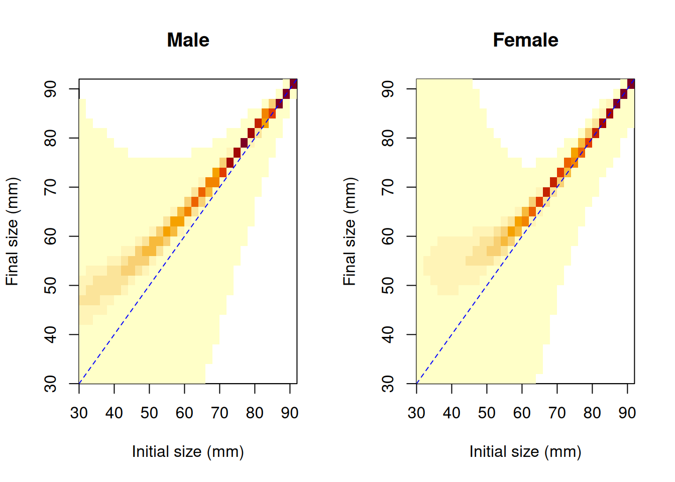
Cross validate growth matrix
Do an experiment / cross validation where we take the initial size (L1) of all tags, then grow them using the growth matrix given their time at liberty, then compare to their size at recapture… how well do we do?
Pretty good match between observed density of L2 and using matrix algebra and model to increment size from L1 to L2.
Try doing this again but using the simulate feature.
isex <- 2
L1 <- data$gi_L1[data$gi_sex == isex]
L2 <- L1 + data$gi_obs[data$gi_sex == isex]
lib <- data$gi_liberty[data$gi_sex == isex]
n_tags <- length(L1)

binwidth <- 1 # mm
a <- seq(30, 92, binwidth)
# a <- c(30, 35, 40, seq(45, 92, binwidth)) # non equal bin widths
mp <- a[-length(a)] + diff(a) / 2
length(mp)

L2_bin <- cut(x = L2, breaks = a) # bin up the data
xx <- table(L2_bin)
xx <- as.numeric(xx / sum(xx))
df_data <- data.frame(L2 = mp, prop = xx)

Lbins <- rep(0, length(mp))
gout <- matrix(NA, nrow = n_tags, ncol = length(mp))

galpha <- exp(opt$par[names(opt$par) %in% "log_galpha"])
gdiff = plogis(opt$par[names(opt$par) %in% "logit_gdiff"])
gbeta <- gdiff * galpha
# gbeta = exp(opt$par[names(opt$par) %in% "log_gbeta"])[isex],

for (i in 1:n_tags) {
  gi <- get_growth_increment(
    midpoint = mp, ga = data$ga, gb = data$gb, gmin = data$gmin,
    galpha = galpha[isex], gbeta = gbeta[isex],
    gshape = exp(opt$par[names(opt$par) %in% "log_gshape"])[isex],
    gcv = exp(opt$par[names(opt$par) %in% "log_gcv"])[isex],
    gobs = 0, gdd = 0, biomass = 1, tau = lib[i])
  gm <- get_growth_matrix(midpoint = mp, increment = gi)
  L1_bin <- cut(x = L1[i], breaks = a, labels = mp)
  L1_vec <- Lbins
  L1_vec[which(mp %in% L1_bin)] <- 1
  gout[i,] <- gm %*% L1_vec
}

L2gm <- colSums(gout)
L2gm <- L2gm / sum(L2gm)
df_pred <- data.frame(L2 = mp, prop = L2gm)

ggplot() +
  # stat_density(aes(x = L2, colour = "Observed L2 dens"),
  # geom = "line", position = "identity") +
  # geom_density(aes(x = L2, colour = "obs_dens"), adjust = 0.5,
  # position = "stack", n = 31) +
  geom_line(data = df_data, aes(x = L2, y = prop, colour = "Observed")) +
  geom_line(data = df_pred, aes(x = L2, y = prop, colour = "Predicted")) +
  labs(x = "TW at recapture (mm)", y = NULL, colour = NULL)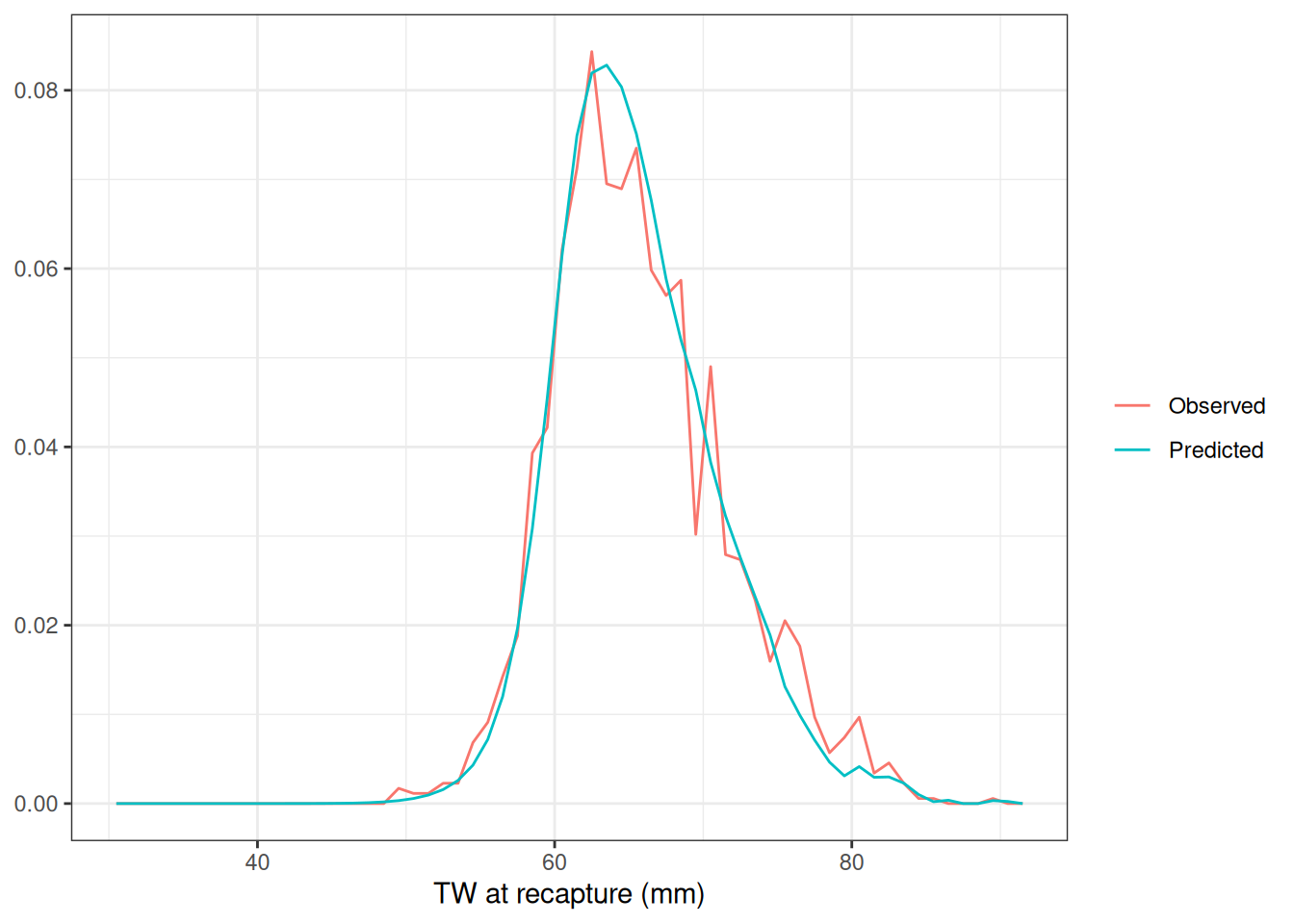
Likelihood profiles
The likelihood-profile helper needs to be expanded so the user can list what to report, as the current version does not work for the growth model.
# lincomb <- numeric(length(names(obj$par)))
# lc <- lincomb; lc[1] <- 1
# # prof_galpha1 <- tmbprofile2(obj = obj, lincomb = lc)
# prof_galpha1 <- TMB::tmbprofile(obj = obj, lincomb = lc)
# lc <- lincomb; lc[2] <- 1
# prof_galpha2 <- TMB::tmbprofile(obj = obj, lincomb = lc)
# plot(prof_galpha1)
# plot(prof_galpha2)
Hilborn, Ray, and Carl J. Walters. 1992. Quantitative Fisheries Stock Assessment: Choice, Dynamics and Uncertainty. Chapman; Hall. https://doi.org/10.1007/978-1-4615-3598-0.
Kristensen, Kasper, Anders Nielsen, Casper W. Berg, Hans Skaug, and Bradley M. Bell. 2016. “TMB: Automatic Differentiation and Laplace Approximation.” Journal of Statistical Software 70 (5): 1–21. https://doi.org/10.18637/jss.v070.i05.
Quinn, Terrance J., and Richard B. Deriso. 1999. Quantitative Fish Dynamics. Oxford University Press.
Schnute, Jon, and David Fournier. 1980. “A New Approach to Estimating Populations and Stock Composition in Mark-Recapture Experiments.” Canadian Journal of Fisheries and Aquatic Sciences 37 (10): 1744–59. https://doi.org/10.1139/f80-220.
Webber, Darcy N., and Robert L. Stephenson. 2016. “A Bayesian Growth Model for Southern Rock Lobster (Jasus Edwardsii) in the New Zealand CRA 2 Management Area.” New Zealand Journal of Marine and Freshwater Research 50 (4): 503–21. https://doi.org/10.1080/00288330.2016.1165374.