
if (dir.exists(file.path("..", "R")) && requireNamespace("pkgload", quietly = TRUE)) {
  pkgload::load_all("..", quiet = TRUE)
} else {
  library(decamod)
}
library(TMBhelper)
library(tidyverse)
library(kableExtra)

theme_set(theme_bw())Load inputs
Below the required R libraries are loaded. The decamod RTMB model is loaded along with several R functions using library(decamod) (Webber and McKenzie 2022, 2024). The kableExtra package is used for generating tables of inputs. The code theme_set(theme_bw()) alters the plot aesthetics. The model is implemented using automatic differentiation via RTMB (Kristensen et al. 2016).
Dimensions
Could have different midpoints by sex. Could have different breaks (i.e., not even). But would probably need to have the same number of length classes? In the future LFs could be estimated to 1mm and then aggregated however the user wants.
# # non equal bin widths - this is what we should aim for
# binwidth <- 2 # mm
# breaks <- c(30, 35, 40, seq(45, 92, binwidth))
# # non equal bin widths - this is to accommodate LFs for aggregation as
# # LFs are in 2mm bins
# binwidth <- 2 # mm
# breaks <- c(30, 34, 38, 42, seq(46, 92, binwidth))
# midpoint_l <- breaks[-length(breaks)] + diff(breaks) / 2
# breaks[length(breaks)] <- Inf
# bins <- cut(x = midpoint_l, breaks = breaks, right = FALSE)

breaks <- c(seq(30, 90, 2), Inf)
bins <- cut(x = seq(31, 91, 2), breaks = breaks, right = FALSE)
midpoint_l <- midcut(seq(31, 91, 2), 30, 92, 2)
bins <- cut(x = midpoint_l, breaks = breaks, right = FALSE)

tibble(bins, midpoint_l) %>% head()
#> # A tibble: 6 × 2
#>   bins    midpoint_l
#>   <fct>        <dbl>
#> 1 [30,32)         31
#> 2 [32,34)         33
#> 3 [34,36)         35
#> 4 [36,38)         37
#> 5 [38,40)         39
#> 6 [40,42)         41
tibble(bins, midpoint_l) %>% tail()
#> # A tibble: 6 × 2
#>   bins     midpoint_l
#>   <fct>         <dbl>
#> 1 [80,82)          81
#> 2 [82,84)          83
#> 3 [84,86)          85
#> 4 [86,88)          87
#> 5 [88,90)          89
#> 6 [90,Inf)         91

tibble(test = c(29, 30, 30.1, 31.9, 32, 35, 90, 91, 91.9, 120)) %>%
  mutate(bin = cut(x = test, breaks = breaks, right = FALSE))
#> # A tibble: 10 × 2
#>     test bin
#>    <dbl> <fct>
#>  1  29   <NA>
#>  2  30   [30,32)
#>  3  30.1 [30,32)
#>  4  31.9 [30,32)
#>  5  32   [32,34)
#>  6  35   [34,36)
#>  7  90   [90,Inf)
#>  8  91   [90,Inf)
#>  9  91.9 [90,Inf)
#> 10 120   [90,Inf)

first_year <- 1945
last_year <- 2023

l_year <- first_year:last_year
l_season <- c("AW", "SS")
l_region <- "CRA 2"
l_sex <- c("Male", "Female")
l_fishery <- c("SL", "NSL")
l_length <- bins
l_cpue <- c("FSU", "CELR", "Logbook")

n_year <- length(l_year)
n_season <- length(l_season)
n_region <- length(l_region)
n_fishery <- length(l_fishery)
n_sex <- length(l_sex)
n_length <- length(midpoint_l)

dim_ytrsl <- c(n_year, n_season, n_region, n_sex, n_length)
dimnames_ytrsl <- list(year = l_year, season = l_season, region = l_region,
                       sex = l_sex, length = l_length)

dim_ytrfl <- c(n_year, n_season, n_region, n_fishery, n_length)
dimnames_ytrfl <- list(year = l_year, season = l_season, region = l_region,
                       fishery = l_fishery, length = l_length)

dim_ytrsfl <- c(n_year, n_season, n_region, n_sex, n_fishery, n_length)
dimnames_ytrsfl <- list(year = l_year, season = l_season, region = l_region,
                        sex = l_sex, fishery = l_fishery, length = l_length)
Tags
Tag-recapture data are used to estimate growth increments following Schnute and Fournier (1980) and Fournier and Archibald (1982).
tags <- tags_CRA2 %>%
  rename(gi_L1 = RelLngth, gi_L2 = RecLngth) %>%
  mutate(gi_obs = gi_L2 - gi_L1, gi_liberty = DaysatLiberty / 365) %>%
  mutate(gi_sex = as.integer(Sex)) %>%
  mutate(gi_morph = gi_sex) %>%
  filter(TagRelease == 0) %>%
  # filter(RelYear %in% first_year:last_year) %>%
  # filter(RecYear %in% first_year:last_year) %>%
  filter(gi_liberty > 0.5, gi_obs > -10)
  # select(gi_sex, gi_morph, gi_L1, gi_liberty, gi_obs)

which_growth_ytrs <- array(0, dim = c(n_year, n_season, n_region, n_sex))
which_growth_ytrs[,,,1] <- 1
which_growth_ytrs[,,,2] <- 2
col.names <- c("Sex", "Initial length (mm)", "Time at liberty (years)",
               "Growth increment (mm)")
tags %>% select(gi_sex, gi_L1, gi_liberty, gi_obs) %>% head(6) %>%
kbl(digits = 1, col.names = col.names,
    caption = "Example tag-recapture records used to estimate growth increments.") %>%
add_header_above(c("Covariates" = 3, "Data" = 1))Catch
catch <- catch_CRA2 %>%
  mutate(SL = Commercial + Recreational, NSL = Illegal + Customary) %>%
  filter(Year >= first_year)

catch_ytrf <- array(0, dim = c(n_year, n_season, n_region, n_fishery),
                    dimnames = list(year = l_year, season = l_season,
                                    region = l_region, fishery = l_fishery))

for (y in 1:n_year) {
  for (t in 1:n_season) {
    if (any(catch$Season == t & catch$Year %in% l_year[y])) {
      catch_ytrf[y,t,1,1] <- catch$SL[catch$Season == t & catch$Year %in% l_year[y]]
      catch_ytrf[y,t,1,2] <- catch$NSL[catch$Season == t & catch$Year %in% l_year[y]]
    }
  }
}
kbl(tail(catch %>% select(-QMA)), digits = 1,
caption = "Recent catch inputs by fishing year, season, and fishery component.")| Year | Season | Commercial | Recreational | Illegal | Customary | SL | NSL |
|---|---|---|---|---|---|---|---|
| 2021 | 1 | 47.5 | 3.2 | 13.5 | 0.5 | 50.7 | 14.0 |
| 2021 | 2 | 32.5 | 28.5 | 9.3 | 4.5 | 61.0 | 13.8 |
| 2022 | 1 | 46.9 | 1.3 | 12.8 | 0.5 | 48.2 | 13.3 |
| 2022 | 2 | 33.1 | 11.6 | 9.0 | 4.5 | 44.7 | 13.5 |
| 2023 | 1 | 36.3 | 1.2 | 11.7 | 0.5 | 37.5 | 12.2 |
| 2023 | 2 | 43.7 | 10.4 | 14.0 | 4.5 | 54.1 | 18.5 |
Legal status and retention
Includes MLS, proportion of females in berry, legal status, and proportion retained:
mls_ytrsfl <- array(1, dim = dim_ytrsfl, dimnames = dimnames_ytrsfl)
for (t in 1:n_season) {
  for (r in 1:n_region) {
    for (y in which(l_year < 1988)) {
      mls_ytrsfl[y, t, r, 1, 1,] <- ifelse(midpoint_l > 53, 1, 0)
      mls_ytrsfl[y, t, r, 2, 1,] <- ifelse(midpoint_l > 58, 1, 0)
    }
    for (y in which(l_year %in% 1988:1991)) {
      mls_ytrsfl[y, t, r, 1, 1,] <- ifelse(midpoint_l > 54, 1, 0)
      mls_ytrsfl[y, t, r, 2, 1,] <- ifelse(midpoint_l > 58, 1, 0)
    }
    for (y in which(l_year > 1991)) {
      mls_ytrsfl[y, t, r, 1, 1,] <- ifelse(midpoint_l > 54, 1, 0)
      mls_ytrsfl[y, t, r, 2, 1,] <- ifelse(midpoint_l > 60, 1, 0)
    }
  }
}

berry_ytrfl <- array(1, dim = dim_ytrfl, dimnames = dimnames_ytrfl)
for (y in 1:n_year) {
  for (t in 1:n_season) {
    sub <- berry_CRA2 %>% filter(Season == t)
    if (nrow(sub) > 0) {
      berry_ytrfl[y,t,,1,] <- 1 - sub$mean_prop_berry
    }
  }
}

legal_ytrsfl <- mls_ytrsfl
for (y in 1:n_year) {
  for (t in 1:n_season) {
    for (r in 1:n_region) {
      for (f in 1:n_fishery) {
        legal_ytrsfl[y,t,r,2,f,] <- legal_ytrsfl[y,t,r,2,f,] * berry_ytrfl[y,t,r,f,]
      }
    }
  }
}

retained_ytrsfl <- array(1, dim = dim_ytrsfl, dimnames = dimnames_ytrsfl)
LFs
Length frequency data are weighted using the iterative re-weighting approach of Francis (2011). For now I have summed over IF and MF and rescaled to 1. I’ve also added code to sum over length bins if needed.
lf <- lf_CRA2 %>%
  arrange(fyear, season, sex) %>%
  mutate(sex = ifelse(sex == 1, 1, 2)) %>%
  mutate(season = ifelse(season == "AW", 1, 2)) %>%
  pivot_longer(cols = starts_with("tw_"), names_to = "length") %>%
  mutate(length = parse_number(length)) %>%
  mutate(bin = cut(x = length, breaks = breaks, right = FALSE)) %>%
  mutate(value = value * weight_scaled) %>%
  group_by(fyear, season, sex, bin) %>%
  summarise(value = sum(value)) %>%
  pivot_wider(names_from = bin, values_from = value) %>%
  ungroup() %>%
  mutate(weight_scaled = rowSums(select(., -c(fyear, season, sex)))) %>%
  relocate(weight_scaled, .after = sex)
lf_obs <- as.matrix(lf %>% select(-c(fyear, season, sex, weight_scaled)))
lf_obs <- lf_obs / rowSums(lf_obs)
Sex ratio
Just using proportion male.
CPUE
Catch per unit effort (CPUE) indices are standardised following Maunder and Punt (2004).
fsu <- fsu_CRA2 %>% mutate(q = 1, units = 0)
celr <- celr_CRA2 %>% mutate(q = 2, units = 0)
logbook <- logbook_CRA2 %>% mutate(q = 3, units = 1)

cpue <- bind_rows(fsu, celr, logbook) %>%
  separate(Year, into = c("year", "season")) %>%
  mutate(year = as.integer(year)) %>%
  mutate(season = as.integer(ifelse(season == "AW", 1, 2))) %>%
  mutate(logSD = log(1 + SD / Mean)) %>%
  mutate(wt = case_when(q == 1 ~ 0.75, q == 2 ~ 1.35, q == 3 ~ 1.31)) %>%
  mutate(pro = 0) # mutate(pro = 0.25)
cpue %>% select(year, season, Median, Mean, SD, logSD, q, units) %>%
  tail(10) %>%
  kbl(digits = 1,
caption = "Recent CPUE index observations and associated uncertainty inputs.")| year | season | Median | Mean | SD | logSD | q | units |
|---|---|---|---|---|---|---|---|
| 2019 | 1 | 1.1 | 1.1 | 0.2 | 0.2 | 3 | 1 |
| 2019 | 2 | 1.4 | 1.4 | 0.3 | 0.2 | 3 | 1 |
| 2020 | 1 | 1.3 | 1.3 | 0.2 | 0.2 | 3 | 1 |
| 2020 | 2 | 1.6 | 1.6 | 0.3 | 0.2 | 3 | 1 |
| 2021 | 1 | 1.4 | 1.4 | 0.2 | 0.2 | 3 | 1 |
| 2021 | 2 | 1.2 | 1.2 | 0.3 | 0.2 | 3 | 1 |
| 2022 | 1 | 1.2 | 1.2 | 0.2 | 0.2 | 3 | 1 |
| 2022 | 2 | 1.3 | 1.3 | 0.3 | 0.2 | 3 | 1 |
| 2023 | 1 | 1.3 | 1.3 | 0.2 | 0.2 | 3 | 1 |
| 2023 | 2 | 1.6 | 1.6 | 0.5 | 0.2 | 3 | 1 |
# plot(cpue$SD, cpue$logSD); abline(coef = c(0, 1), col = 2)
# plot(cpue$CV, cpue$logSD); abline(coef = c(0, 1), col = 2)
x <- seq(0.32, 0.43, length.out = 10)
wt <- 1.2
y <- sqrt(x^2 + 0.25^2) * 1.0 / wt
plot(x)
lines(y, col = 2) # effect of adding process error is to make sds more similar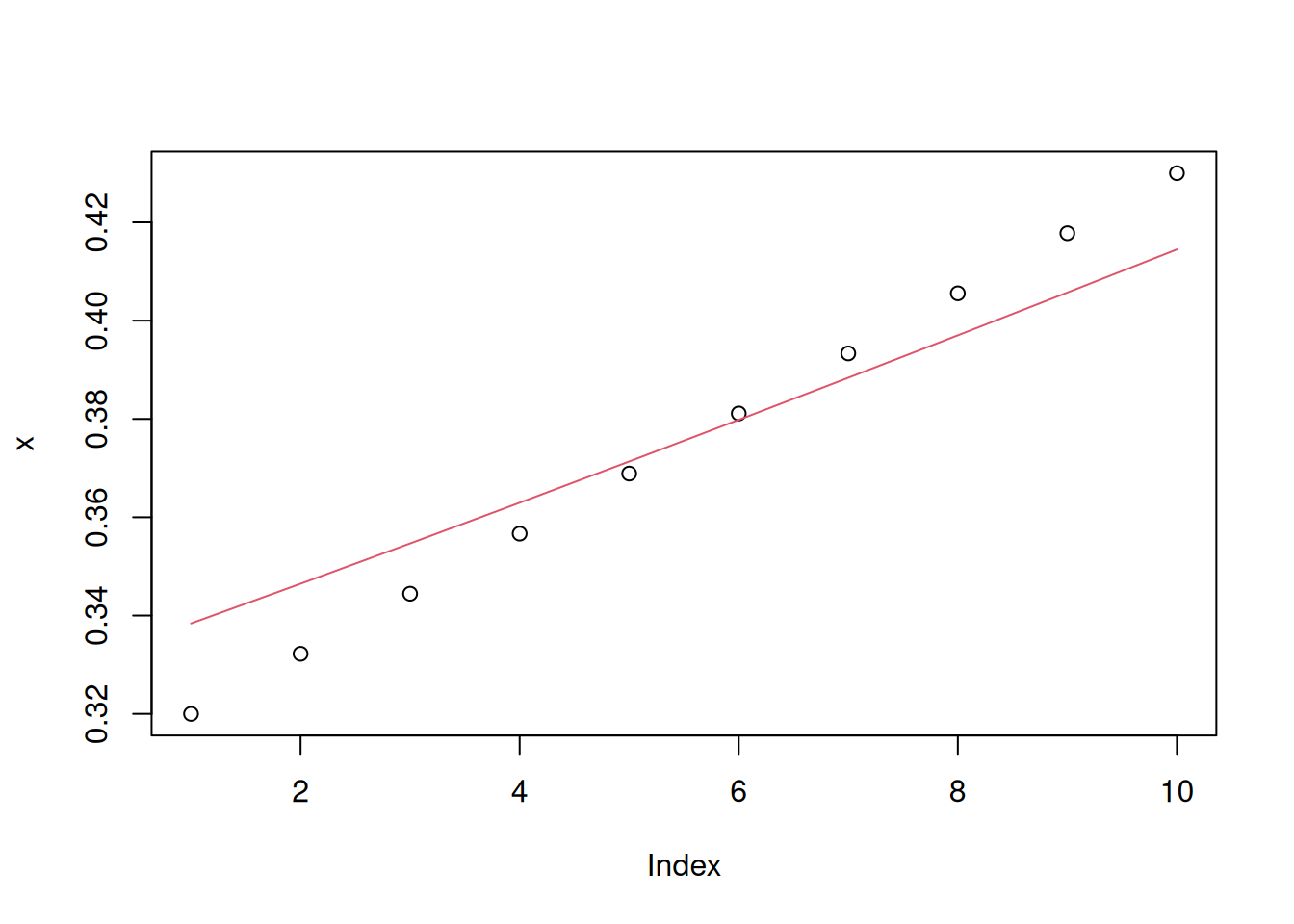
Maturity
Maturity is set to zero for males.
maturity_ytrsl <- array(0, dim = dim_ytrsl, dimnames = dimnames_ytrsl)
for (y in 1:n_year) {
  for (t in 1:n_season) {
    for (r in 1:n_region) {
      maturity_ytrsl[y,t,r,2,] <- logistic_ogive(x = midpoint_l,
                                                 x50 = 50.4482, x95 = 11.2724)
    }
  }
}
as.data.frame(ftable(maturity_ytrsl)) %>%
  filter(year == last_year, season == "AW", sex == "Female") %>%
  ggplot(aes(x = length, y = Freq)) +
  geom_point() +
  scale_y_continuous(limits = c(0, 1)) +
  labs(x = "Tail width bin (mm)", y = "Proportion mature") +
  theme(axis.text.x = element_text(angle = 45, vjust = 1, hjust = 1))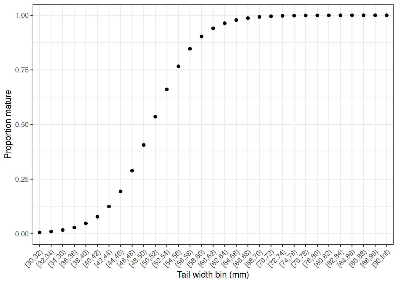
Weight
weight_a <- c(4.16e-06, 1.30e-05)
weight_b <- c(2.9354, 2.5452)
n_weight <- length(weight_a)

which_weight_ytrs <- array(0, dim = c(n_year, n_season, n_region, n_sex))
which_weight_ytrs[,,,1] <- 1
which_weight_ytrs[,,,2] <- 2

weight_il <- matrix(0, nrow = n_weight, ncol = n_length)
for (i in 1:n_weight) {
  weight_il[i,] <- length_to_weight(midpoint_l, weight_a[i], weight_b[i])
}

weight_ytrsl <- get_weight(weight_il, which_weight_ytrs)
dimnames(weight_ytrsl) <- dimnames_ytrsl
plot(midpoint_l, weight_ytrsl[1,1,1,1,], type = "l", col = 4)
lines(midpoint_l, weight_ytrsl[1,1,1,2,], type = "l", col = 2)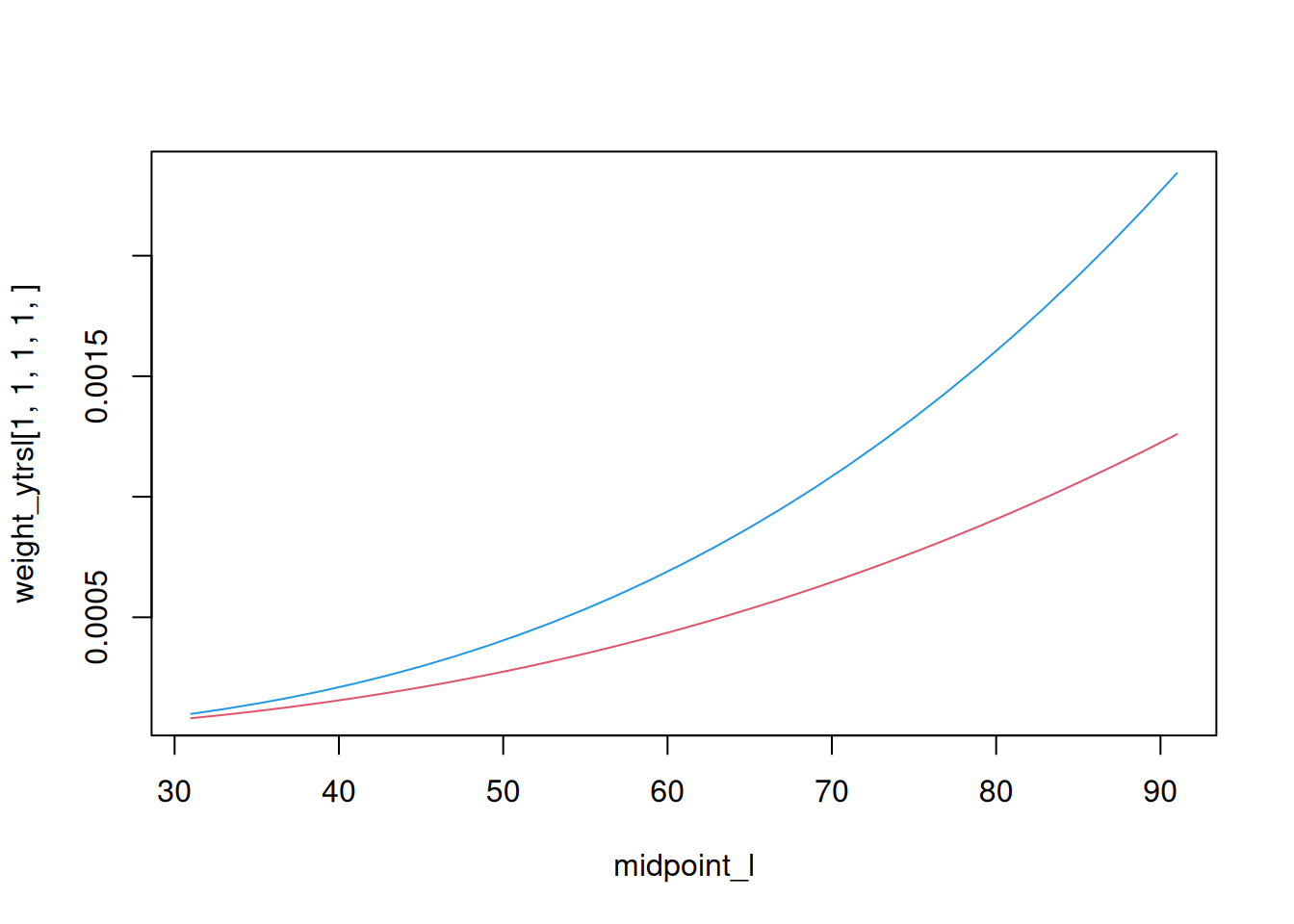
Is M at midpoints same as M integrated over lengths try v small bins vs large bins.
midpoint2 <- seq(31, 91, 2)
M2 <- get_M_length(midpoint2, a = 60, Ma = 0.2, Mc = -1)
df2 <- tibble(midpoint2 = midpoint2, M = M2, N = 10000) %>%
  mutate(NeM = N * exp(-M))

midpoint1 <- seq(31, 92, 1)
M1 <- get_M_length(midpoint1, a = 60, Ma = 0.2, Mc = -1)
df1 <- tibble(midpoint1 = midpoint1, M = M1, N = 5000) %>%
  mutate(NeM = N * exp(-M)) %>%
  mutate(id = cut(x = midpoint1, breaks = seq(30, 92, 2), labels = FALSE)) %>%
  mutate(midpoint2 = midpoint2[id]) %>%
  group_by(midpoint2) %>%
  summarise(N = sum(N), NeM = sum(NeM))

sum(df1$N)
#> [1] 310000
sum(df2$N)
#> [1] 310000
sum(df1$NeM)
#> [1] 250700.3
sum(df2$NeM)
#> [1] 250191.4

plot(midpoint2, df1$NeM, type = "l")
lines(midpoint2, df2$NeM, col = 2)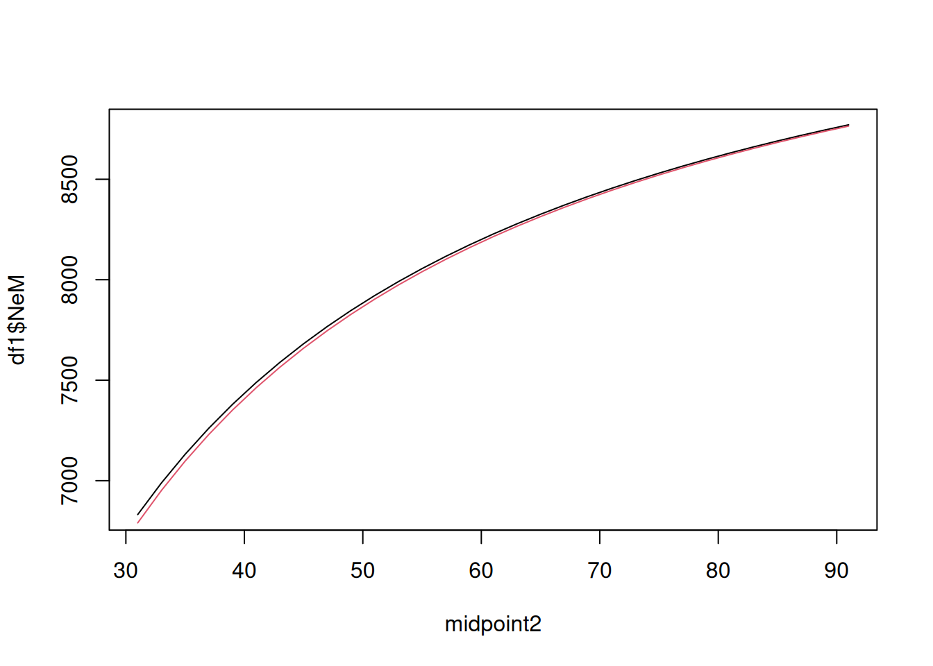
Selectivity
Selectivity is modelled as a double-normal ogive (Quinn and Deriso 1999).
Define data list
Define the data list that can be passed to MakeADFun:
data <- list(
  first_year = first_year,
  n_year = n_year, n_season = n_season, n_region = n_region, n_sex = n_sex,
  n_fishery = n_fishery,
  midpoint_l = as.numeric(midpoint_l),
  l_year = l_year, l_season = l_season, l_region = l_region, l_sex = l_sex,
  l_fishery = l_fishery, l_length = l_length, l_cpue = l_cpue,
  weight_ytrsl = weight_ytrsl, maturity_ytrsl = maturity_ytrsl,
  # Selectivty
  n_sel = 4, # M AW, F AW, M SS, F SS
  sel_like = 0, # 0=off, 1=RE
  # sel_type = c(1, 2, 1, 2), # 0=constant 1, 1=logistic, 2=logistic-capped
  sel_type = c(2, 2, 2, 2), # 0=constant 1, 1=logistic, 2=logistic-capped
  which_sel_ytrsf = which_sel_ytrsf,
  # M
  M_size = 60,
  which_M_ytrs = array(1, dim = c(n_year, n_season, n_region, n_sex)),
  # Recruitment
  rec_like = 5, # 0=off, 1=RE, 2=RW, 3=AR1, 4=RE/RW, 5=RE/AR1
  rsigma_bias = 0,
  last_rdev_year = n_year,
  # Growth
  # 1=Francis, 2=generalized Linf/K/gamma, 3=constrained reference,
  # 4=fixed external mean, 5=integrated monotone ODE
  growth_model = 1,
  growth_transition = 1, # 1=legacy finite-time Normal, 2=continuous-time latent process
  growth_like = 3, # 0=off, 1=normal, 2=robust-normal (historical), 3=student-t
  growth_df = 3, # Student-t degrees of freedom; gi_sd is its actual SD
  growth_dd = 1, # density dependent growth: 0=off, 1=on
  n_growth = 2,
  n_tags = nrow(tags),
  ga = 50, gb = 80,
  gmin = 0.0001, # gmin = -10,
  which_growth_ytrs = which_growth_ytrs,
  # need which statements for each growth parameter
  # Catch
  catch_like = -1, # -1=Us, 0=Fs using NR, 1=normal, 2=lognormal
  catch_obs = as.vector(catch_ytrf),
  catch_cv = 0.06,
  pen_wt = 1000,
  match_old_u = 0,
  catch_ytrf = catch_ytrf,
  mls_ytrsfl = mls_ytrsfl,
  legal_ytrsfl = legal_ytrsfl,
  retained_ytrsfl = retained_ytrsfl,
  handling_mortality_y = ifelse(l_year < 1990, 0.1, 0.05),
  # CPUE
  cpue_like = 2, # 0=off, 1=normal, 2=lognormal, 3=gamma
  cpue_first_qcreep = c(1990, 1990, 1993) - first_year + 1,
  cpue_obs = cpue$Median,
  cpue_sd = cpue$logSD,
  cpue_pro = cpue$pro,
  cpue_wt = c(0.75, 0.7, 1)[cpue$q],
  cpue_q = cpue$q,
  cpue_units = cpue$units, # 0=numbers, 1=weight
  cpue_fishery = rep(1, nrow(cpue)),
  cpue_year = cpue$year - first_year + 1,
  cpue_season = cpue$season, # AW, SS
  cpue_region = rep(1, nrow(cpue)),
  cpue_sex = rep(0, nrow(cpue)), # 0=all, 1=female, 2=male
  # Sex-ratio
  sexr_like = 2, # 0=off, 1=old, 2=logit-normal, 3=beta
  sexr_obs = sexr$mean_scaled_1,
  sexr_sd = sexr$weight_scaled,
  sexr_wt = rep(800, nrow(sexr)),
  sexr_year = sexr$fyear - first_year + 1,
  sexr_season = sexr$season,
  sexr_region = rep(1, nrow(sexr)),
  sexr_fishery = rep(1, nrow(sexr)),
  # LFs
  lf_like = 1, # 1=multinomial, 2=Dirichlet
  lf_obs = lf_obs,
  lf_min = rep(8, nrow(lf)),
  lf_max = rep(n_length - 4, nrow(lf)),
  # lf_max = rep(n_length - 1, nrow(lf)),
  lf_roll = rep(1, nrow(lf)),
  lf_sd = lf$weight_scaled,
  lf_wt = ifelse(lf$sex == 1, 1.204, 0.982),
  lf_year = lf$fyear - first_year + 1,
  lf_season = lf$season,
  lf_region = rep(1, nrow(lf)),
  lf_sex = lf$sex,
  lf_fishery = rep(1, nrow(lf)),
  # Switches
  jacobian_on = 0, prior_on = 1, like_on = 1)

data <- c(data, as.list(tags))
names(data)
#>   [1] "first_year"           "n_year"               "n_season"
#>   [4] "n_region"             "n_sex"                "n_fishery"
#>   [7] "midpoint_l"           "l_year"               "l_season"
#>  [10] "l_region"             "l_sex"                "l_fishery"
#>  [13] "l_length"             "l_cpue"               "weight_ytrsl"
#>  [16] "maturity_ytrsl"       "n_sel"                "sel_like"
#>  [19] "sel_type"             "which_sel_ytrsf"      "M_size"
#>  [22] "which_M_ytrs"         "rec_like"             "rsigma_bias"
#>  [25] "last_rdev_year"       "growth_model"         "growth_transition"
#>  [28] "growth_like"          "growth_df"            "growth_dd"
#>  [31] "n_growth"             "n_tags"               "ga"
#>  [34] "gb"                   "gmin"                 "which_growth_ytrs"
#>  [37] "catch_like"           "catch_obs"            "catch_cv"
#>  [40] "pen_wt"               "match_old_u"          "catch_ytrf"
#>  [43] "mls_ytrsfl"           "legal_ytrsfl"         "retained_ytrsfl"
#>  [46] "handling_mortality_y" "cpue_like"            "cpue_first_qcreep"
#>  [49] "cpue_obs"             "cpue_sd"              "cpue_pro"
#>  [52] "cpue_wt"              "cpue_q"               "cpue_units"
#>  [55] "cpue_fishery"         "cpue_year"            "cpue_season"
#>  [58] "cpue_region"          "cpue_sex"             "sexr_like"
#>  [61] "sexr_obs"             "sexr_sd"              "sexr_wt"
#>  [64] "sexr_year"            "sexr_season"          "sexr_region"
#>  [67] "sexr_fishery"         "lf_like"              "lf_obs"
#>  [70] "lf_min"               "lf_max"               "lf_roll"
#>  [73] "lf_sd"                "lf_wt"                "lf_year"
#>  [76] "lf_season"            "lf_region"            "lf_sex"
#>  [79] "lf_fishery"           "jacobian_on"          "prior_on"
#>  [82] "like_on"              "Event"                "Sex"
#>  [85] "RelMonth"             "RelYear"              "RecMonth"
#>  [88] "RecYear"              "DaysatLiberty"        "gi_L1"
#>  [91] "gi_L2"                "TWConvertRel"         "TWConvertRec"
#>  [94] "TagRelease"           "RelStatArea"          "Condition"
#>  [97] "Tagtype"              "RecStatArea"          "gi_obs"
#> [100] "gi_liberty"           "gi_sex"               "gi_morph"
# sqrt(data$cpue_sd^2 + data$cpue_pro^2) / data$cpue_wt # cpue_sigma
# hist(rlnorm(n = 10000, meanlog = log(2), sdlog = sqrt(data$cpue_sd^2 + data$cpue_pro^2) / data$cpue_wt))
# ii <- 11
# yy <- data$lf_obs[ii,4:31] / sum(data$lf_obs[ii,4:31])
# xx <- gtools::rdirichlet(n = 10000, alpha = yy * data$lf_sd[ii] * data$lf_wt[ii])
# plot(yy, type = "b", col = 2, ylim = c(0, 0.25))
# for (i in 1:100) lines(xx[i,] / sum(xx[i,]), col = 4)
# data$lf_obs <- round(data$lf_obs[,data$lf_min[1]:data$lf_max[1]] * data$lf_sd * data$lf_wt)
# data$lf_N <- rowSums(data$lf_obs)
Model setup
Define the parameter list:
parameters <- list(
  log_F0 = log(0), logit_U0 = qlogis(1e-06),
  log_R0 = log(554439), log_Rsigma = log(0.25), Rrho = 0,
  logit_h = qlogis(0.999), log_Rmu = log(32), log_Rsd = log(2),
  log_Ma = log(c(0.187377, 0.187377)), Mc = c(0, 0), #Mc = -1,
  log_q = log(c(0.00127899, 0.00242722, 1.27082e-06)),
  log_pow = c(0, 0, 0),
  qcreep = c(0.01, 0.01, 0.01),
  log_galpha = log(c(6.89278, 4.98873)),
  logit_gdiff = qlogis(c(0.351061,  0.229016)),
  log_gshape = log(c(1.78938, 4.03173)),
  log_gcv = log(c(0.428625, 0.731757)),
  log_gobs = log(1.05115),
  log_gdd = log(0),
  log_sel50 = log(c(50.8998, 55.5424, 50.8998, 55.5424)),
  log_sel95 = log(c(4.68424, 7.56075, 4.68424, 7.56075)),
  log_seldome = log(c(1, 1, 1, 1)),
  log_selmax = log(c(1, 0.5904295, 1, 0.724695)),
  sel_sd50 = 0.1, sel_sd95 = 0.1, sel_sdmax = 0.1,
  N0dev = rep(0, n_region * n_sex * n_length),
  log_F = rep(log(0.02), length(data$catch_ytrf)),
  Rdev_yr = array(c(
    rep(0.5, 34),
    0.443867, 0.13716, 0.309184, 0.374968, 0.162059, 0.0988453,
    0.0256326, -0.1596, -0.138787, -0.144103, -0.137282, 0.220984, 0.573551,
    0.766394, 0.57366, 0.188741, -0.205083, -0.452905, -0.412874, -0.403783,
    -0.511264, -0.0934694, -0.0812145, -0.144924, 0.335367, -0.0463576,
    -0.147839, -0.065563, -0.13226, -0.400957, 0.193345, -0.0966899, -0.379127,
    -0.46455, -0.513768, -0.382686, 0.256375, -0.114664, -0.451873, -0.369532,
    -0.362545, -0.789267, rep(-0.789267, 3)), dim = c(n_year, n_region))
)
Generalized Linf/K/gamma growth option
The integrated assessment can use the same deterministic Schnute–Francis family in generalized coordinates by setting growth_model = 2. This is a reparameterization of the mean curve, not a new biological growth family. It makes the asymptote and rate explicit and uses model-internal transforms that require to exceed the fitted length domain, , and . Those restrictions prevent the expected increment curve from turning upward with length.
The fitted parameters are log_linf_excess, log_growth_rate, and shape_unconstrained; decamod() reports natural-scale linf, k (also available as growth_rate), and gshape. The following shows the alternative setup. It replaces, rather than supplements, log_galpha, logit_gdiff, and log_gshape.
data$growth_model <- 2
data$growth_shape_lower <- 1
data$growth_shape_upper <- 8
data$growth_linf_floor <- vapply(seq_len(data$n_growth), function(group) {
  tag_rows <- data$gi_morph == group
  max(c(data$midpoint_l, data$gi_L1[tag_rows]), na.rm = TRUE) + 1
}, numeric(1))

parameters$log_galpha <- NULL
parameters$logit_gdiff <- NULL
parameters$log_gshape <- NULL
parameters$log_linf_excess <- rep(log(15), data$n_growth)
parameters$log_growth_rate <- rep(log(0.08), data$n_growth)
parameters$shape_unconstrained <- rep(
  qlogis((2 - data$growth_shape_lower) /
    (data$growth_shape_upper - data$growth_shape_lower)),
  data$n_growth
)

growth_priors <- get_priors(
  parameters,
  growth_shape_lower = data$growth_shape_lower,
  growth_shape_upper = data$growth_shape_upper,
  growth_shape_prior_mean = 2
)
No Jacobian is added: these priors are declared directly on the three sampled coordinates. A Jacobian would be needed only to preserve a prior density first defined on a different parameterization.
Selected monotone-ODE growth options
The selected all-QMA monotone ODE can enter an assessment in two deliberately different ways. The primary fixed/cut implementation sets growth_model = 4. The external growth fit is first used to calculate the expected increment at every population-bin midpoint, every observed tag release length, and the two reference lengths. Those three arrays are fixed in the assessment, while decamod applies the historical finite-time growth matrix and the selected length-diffusion variance. If the target-area tags conditioned the external curve, set growth_like = 0 so they are not counted twice.
data$growth_model <- 4L
data$growth_transition <- 1L
data$growth_variance <- 2L
data$growth_like <- 0L
data$growth_fixed_population_increment <- external_curve$population
data$growth_fixed_tag_increment <- external_curve$tag
data$growth_fixed_reference_increment <- external_curve$reference

parameters$log_galpha <- NULL
parameters$logit_gdiff <- NULL
parameters$log_gshape <- NULL
parameters$log_gsigma <- log(external_curve$sigma60)
The secondary integrated-prior implementation sets growth_model = 5. Its parameter is a 19-coordinate vector: five baseline-shape logits per sex, four local coordinates per sex (log(B50), adult tilt, low-size tilt, and log(sigma60)), and one log(Gobs) coordinate. Males and females use the same ODE equation, knot basis, integration method, support rule, and parameter bounds; their coordinate values may differ. The joint Normal prior is supplied through its mean, precision matrix, and covariance log determinant. A leave-target-area-out predictive prior can use all 19 coordinates and retain the target-area tag likelihood. Alternatively, when the upstream analysis already includes those tags, the downstream tag likelihood must be off. In that cut formulation, growth_ode_prior_index identifies the subset of the 19 coordinates governed by the joint prior; structurally fixed or irrelevant coordinates are fixed with the usual RTMB parameter map.
data$growth_model <- 5L
data$growth_transition <- 1L
data$growth_variance <- 2L
data$growth_like <- 3L
data$growth_df <- 3
data$growth_ode_knot <- c(30, 40, 50, 65, 80, 100)
data$growth_ode_width <- 6
data$growth_ode_floor <- 0.02
data$growth_ode_steps <- 24L
data$growth_ode_adult_contrast <- c(0, 0, 0, -1, 0, 1)
data$growth_ode_low_contrast <- c(1, 0, -1, 0, 0, 0)
data$growth_ode_prior_mean <- external_prior$mean
data$growth_ode_prior_index <- external_prior$growth_ode_prior_index
data$growth_ode_prior_precision <- solve(external_prior$covariance)
data$growth_ode_prior_log_determinant <- as.numeric(
  determinant(external_prior$covariance, logarithm = TRUE)$modulus
)

parameters[c(
  "log_galpha", "logit_gdiff", "log_gshape", "log_gcv",
  "log_gsigma", "log_gobs"
)] <- NULL
parameters$growth_ode_coordinate <- external_prior$parameter_template
get_growth_increment_ode() exposes the same deterministic ODE mean for checking curves and constructing fixed inputs. In an integrated fit, every marginal and joint prior-to-posterior movement in the active coordinates should be reported against the fixed/cut result.
Optional continuous-time growth transition
The historical finite-time Normal population matrix remains the default (growth_transition = 1). With generalized growth coordinates, an assessment can instead opt into the finite-state continuous-time latent process using growth_transition = 2. Its column-oriented generator has non-negative off-diagonal rates and zero column sums, and the population transition is
Consequently to numerical precision. The generator includes rates to shorter states, so biological shrinkage remains possible. gcv controls latent process spread, while gobs is kept out of the population matrix.
Tag releases are represented by linear interpolation between adjacent length states. Their liberty intervals are rounded to a regular grid so transition matrices can be reused. Under the recommended Student- likelihood, the latent state probabilities are integrated against a Student- observation density whose actual SD is gobs; the heavy tails are therefore an observation/outlier model rather than a biological movement kernel.
data$growth_model <- 2
data$growth_transition <- 2
data$growth_like <- 3
data$growth_df <- 3
data <- prepare_growth_transition_data(data, time_step = 1 / 12)
The option currently requires equally spaced length states, positive mean drift over the modelled range, and growth_like equal to 0, 1, or 3. The historical robust Normal likelihood remains available with the legacy matrix for reproducibility, but is not a valid observation mixture and is therefore not enabled for the continuous-time option.
The finite-state upwind approximation adds grid-scale numerical diffusion. Away from the boundaries its infinitesimal second moment is , where is the target diffusion variance rate, is drift, and is length-state spacing. Check sensitivity to a finer internal grid before using the option operationally.
priors <- list()
priors[["logit_U0"]] <- list(type = "normal", par1 = 0, par2 = 1.5, index = which("logit_U0" == names(parameters)))
priors[["log_Ma"]] <- list(type = "normal", par1 = log(0.12), par2 = 0.4, index = which("log_Ma" == names(parameters)))
priors[["log_galpha"]] <- list(type = "normal", par1 = log(2), par2 = 1.655705, index = which("log_galpha" == names(parameters))) # matches dnorm(2, 30)
priors[["logit_gdiff"]] <- list(type = "normal", par1 = -2, par2 = 1.5, index = which("logit_gdiff" == names(parameters)))
priors[["log_gshape"]] <- list(type = "normal", par1 = c(log(4.81), log(4.51)), par2 = c(0.2016748, 0.2142224), index = which("log_gshape" == names(parameters))) # matches dnorm(4.81, 1), dnorm(4.51, 1)
priors[["log_gcv"]] <- list(type = "normal", par1 = c(log(0.59), log(0.82)), par2 = c(0.439544, 0.3360953), index = which("log_gcv" == names(parameters))) # matches dnorm(0.59, 0.3), dnorm(0.82, 0.3)
priors[["log_gobs"]] <- list(type = "normal", par1 = log(1.48), par2 = 0.04990982, index = which("log_gobs" == names(parameters))) # matches dnorm(1.48, 0.074)
priors[["log_Rmu"]] <- list(type = "normal", par1 = log(32), par2 = 0.1, index = which("log_Rmu" == names(parameters)))
priors[["log_Rsd"]] <- list(type = "normal", par1 = log(2), par2 = 0.1, index = which("log_Rsd" == names(parameters)))
priors[["log_Rsigma"]] <- list(type = "normal", par1 = log(0.4), par2 = 0.3, index = which("log_Rsigma" == names(parameters)))
priors[["log_sel50"]] <- list(type = "normal", par1 = log(50), par2 = 0.5, index = which("log_sel50" == names(parameters))) # matches dnorm(50, 30)
priors[["log_sel95"]] <- list(type = "normal", par1 = log(10), par2 = 1.124519, index = which("log_sel95" == names(parameters))) # matches dnorm(10, 30)
priors[["log_selmax"]] <- list(type = "normal", par1 = -log(2) / 2, par2 = sqrt(log(2)), index = which("log_selmax" == names(parameters)))
data <- c(data, priors)
Use TMB’s map option to turn parameters on/off:
map <- list()
map[["log_F0"]] <- factor(NA)
map[["logit_U0"]] <- factor(NA)
map[["logit_h"]] <- factor(rep(NA, length(parameters$logit_h)))
map[["N0dev"]] <- factor(rep(NA, length(parameters$N0dev)))
map[["log_Rsigma"]] <- factor(NA)
map[["Rrho"]] <- factor(NA)
map[["log_Rmu"]] <- factor(NA)
map[["log_Rsd"]] <- factor(NA)
map[["log_Ma"]] <- factor(c(1, 1))
map[["Mc"]] <- factor(rep(NA, length(parameters$Mc)))
map[["qcreep"]] <- factor(rep(NA, length(parameters$qcreep)))
# map[["log_pow"]] <- factor(c(NA, 1, 2))
map[["log_pow"]] <- factor(c(NA, NA, NA))
map[["log_gdd"]] <- factor(NA)
map[["log_sel50"]] <- factor(c(1, 2, 1, 2))
map[["log_sel95"]] <- factor(c(1, 2, 1, 2))
map[["log_selmax"]] <- factor(c(NA, 1, 2, 3))
map[["log_seldome"]] <- factor(c(NA, NA, NA, NA))
map[["sel_sd50"]] <- factor(NA)
map[["sel_sd95"]] <- factor(NA)
map[["sel_sdmax"]] <- factor(NA)
map[["log_F"]] <- factor(rep(NA, length(parameters$log_F)))
Year-, sex-, and length-specific deviations can optionally be applied to the baseline selectivity curves. Supply log_sels and log_selvar together; log_sels must have dimensions year by sex by length. The deviations are multiplied onto each matching selectivity curve and receive a zero-centred normal prior with standard deviation exp(log_selvar).
Create the AD object using TMBs MakeADFun function from the TMB framework (Kristensen et al. 2016):
# check_data(data = data, parameters = parameters)
# obj <- MakeADFun(func = cmb(decamod, data), parameters = parameters, map = map, random = "Rdev_yr")
# data$rec_like <- 1 # 0=off, 1=RE, 2=RW, 3=AR1, 4=RE/RW, 5=RE/AR1
obj <- MakeADFun(func = cmb(decamod, data), parameters = parameters, map = map)
Optimisation
List of parameters that are on:
The objective function value given the initial values:
obj$fn(obj$par)
#> [1] 12489.26
Load the default parameter bounds:
Lwr <- rep(-Inf, length(obj$par))
Upr <- rep(Inf, length(obj$par))

Lwr[grep("log_R0", names(obj$par))] <- 1
Upr[grep("log_R0", names(obj$par))] <- 25
Lwr[grep("log_Ma", names(obj$par))] <- log(0.01)
Upr[grep("log_Ma", names(obj$par))] <- log(0.35)
Lwr[grep("log_q", names(obj$par))] <- -25
Upr[grep("log_q", names(obj$par))] <- 1
Lwr[grep("log_galpha", names(obj$par))] <- log(0)
Upr[grep("log_galpha", names(obj$par))] <- log(15)
Lwr[grep("logit_diff", names(obj$par))] <- qlogis(0.001)
Upr[grep("logit_diff", names(obj$par))] <- qlogis(0.99)
Lwr[grep("log_gshape", names(obj$par))] <- log(0.1)
Upr[grep("log_gshape", names(obj$par))] <- log(10)
Lwr[grep("log_gcv", names(obj$par))] <- log(0.01)
Upr[grep("log_gcv", names(obj$par))] <- log(2)
Lwr[grep("log_gobs", names(obj$par))] <- log(0.00001)
Upr[grep("log_gobs", names(obj$par))] <- log(5)
Lwr[grep("log_sel50", names(obj$par))] <- log(30)
Upr[grep("log_sel50", names(obj$par))] <- log(80)
Lwr[grep("log_sel95", names(obj$par))] <- log(1)
Upr[grep("log_sel95", names(obj$par))] <- log(50)
Lwr[grep("log_selmax", names(obj$par))] <- log(0.01)
Upr[grep("log_selmax", names(obj$par))] <- log(2)
Lwr[grep("Rdev_yr", names(obj$par))] <- -2.3
Upr[grep("Rdev_yr", names(obj$par))] <- 2.3

bounds <- data.frame(par = names(obj$par), lower = Lwr, value = obj$par, upper = Upr)
Optimise using the nlminb function:
control <- list(eval.max = 100000, iter.max = 100000)
# opt <- nlminb(start = obj$par, objective = obj$fn, gradient = obj$gr, hessian = obj$he, control = control, lower = bounds$lower, upper = bounds$upper)
# opt <- nlminb(start = opt$par, objective = obj$fn, gradient = obj$gr, hessian = obj$he, control = control, lower = bounds$lower, upper = bounds$upper)
# check_estimability(obj = obj)
# save(data, parameters, bounds, map, obj, opt, file = "inst/extdata/opt.rda")
load(system.file("extdata", "opt.rda", package = "decamod"))
obj_orig <- obj
obj <- MakeADFun(func = cmb(decamod, data), parameters = parameters, map = map)
obj$par <- obj_orig$env$last.par.best
obj$env$last.par <- obj_orig$env$last.par.best
obj$env$last.par.best <- obj_orig$env$last.par.best
sim_check <- obj$simulate(par = obj$env$last.par.best)
sim_check$cpue_obs
#> [1] 1.1061537 2.1093838 1.2622402 1.3965425 1.1538223 1.3111213 0.7719371
#> [8] 1.0865787 0.6851478 1.2530472 0.7741262 1.0536573 0.8069666 1.0241568
#> [15] 0.8580419 0.8792655 0.8304345 0.7892556 0.7995159 0.8360748 0.6611205
#> [22] 1.0901952 1.0718549 0.9853159 1.1247051 0.9544349 0.7707362 1.0392414
#> [29] 1.2633632 0.7110500 1.4424089 1.3357780 1.3941030 2.2137840 1.8289262
#> [36] 2.7518350 1.6659237 1.1467627 1.4634798 1.6057154 2.3900200 1.2776482
#> [43] 1.2970752 0.9503213 1.1308401 0.9382643 1.1113349 0.7497266 1.1124630
#> [50] 0.8507861 1.0092650 0.7034055 0.7118237 1.1356084 0.8840265 0.6637069
#> [57] 1.1045511 0.8193257 1.1715883 0.8929045 0.8700957 0.7603808 1.0834412
#> [64] 0.6100185 0.6503102 0.6326619 0.8659932 0.7169631 1.3343854 0.5760194
#> [71] 0.7938197 0.6076106 0.9364921 0.4543161 0.6115757 0.6581946 0.6979938
#> [78] 1.2167051 1.2507129 1.4025213 0.7739954 1.0118261 0.8970969 1.2618674
#> [85] 1.5814329 1.6347701 1.5563624 1.4019519 2.2463790 2.1562309 1.2618257
#> [92] 1.4846712 0.9777928 1.2919084 1.3122282 1.1723032 0.8857912 1.0055097
#> [99] 0.7295796 0.7956155 0.7687822 0.9059808 0.6914697 1.1521843 0.6918058
#> [106] 1.1502031 0.7886882 0.7346665 1.0308649 1.2611677 0.6648698 0.9038239
#> [113] 0.7117075 0.8483143 0.7444535 1.2162406 0.7893815 0.9828826 0.6605985
#> [120] 0.7157806 0.7049519 0.8302224 0.5377311 0.9063164 0.5832888 0.7314669
#> [127] 0.6896189 0.6886140 0.4589805 0.7765702 0.9248340 0.9466154 1.1022795
#> [134] 1.1027067 1.2305872 1.1494382 1.2833265 1.1805851 1.2153757 1.4471711
#> [141] 1.5453662 1.8482072
sim_check$sexr_obs2
#> [1] 0.208361290 -0.226171780 0.325120628 0.093302359 0.520916957
#> [6] 0.016023777 0.344913305 0.092479255 0.427435910 -0.012225019
#> [11] 0.310104554 -0.373507615 -0.151364593 -0.365536629 -0.121172541
#> [16] -0.498060803 0.119529446 -0.113792669 -0.081566548 -0.434583699
#> [21] 0.068237154 -0.446390284 0.012102095 -0.304006054 0.184434920
#> [26] -0.089823474 0.251015042 -0.153515497 0.077748840 -0.034561519
#> [31] 0.247952172 -0.211752239 0.247512941 -0.229006838 -0.350042442
#> [36] -0.218303759 0.126367077 -0.122470173 0.050939919 -0.183695100
#> [41] 0.169178525 -0.360625141 0.090349799 -0.447512911 0.033806199
#> [46] -0.029527178 0.059569840 -0.361191828 0.137610767 -0.313900584
#> [51] 0.231343944 -0.183826796 0.446010399 -0.251144391 0.422341899
#> [56] -0.009165975 0.324382391 0.064677296 0.368662891 -0.151729324
#> [61] 0.415502534 0.052367950
sim_check$lf_obs2
#> [,1] [,2] [,3] [,4] [,5] [,6] [,7] [,8] [,9] [,10] [,11] [,12] [,13]
#> [1,] 0 2 6 10 9 10 5 6 9 5 4 2 3
#> [2,] 2 0 0 5 7 12 6 7 10 12 4 2 5
#> [3,] 0 1 6 8 13 13 18 13 5 10 6 1 1
#> [4,] 2 2 4 7 11 12 10 17 15 6 8 7 4
#> [5,] 2 1 4 12 12 24 18 12 9 7 3 3 2
#> [6,] 2 1 3 5 8 12 12 17 9 21 9 5 7
#> [7,] 0 1 3 7 6 21 15 9 11 13 3 5 5
#> [8,] 1 1 4 9 7 12 14 13 14 10 10 8 3
#> [9,] 1 1 2 7 19 15 14 9 8 4 5 1 2
#> [10,] 1 1 2 1 5 7 9 11 10 14 6 6 2
#> [11,] 0 0 1 3 5 18 14 8 10 7 6 1 2
#> [12,] 0 2 1 1 7 8 4 6 15 9 4 6 5
#> [13,] 0 0 3 3 14 14 11 10 13 6 8 5 3
#> [14,] 0 0 0 2 5 10 9 12 9 10 10 7 4
#> [15,] 1 0 0 7 11 9 6 8 3 6 10 6 7
#> [16,] 1 1 1 1 4 7 7 13 13 9 6 3 1
#> [17,] 0 2 1 4 10 3 11 10 9 8 6 7 3
#> [18,] 0 1 0 2 4 4 7 7 8 9 9 8 2
#> [19,] 0 0 2 7 7 10 6 6 4 4 11 2 2
#> [20,] 0 0 2 1 1 8 4 4 8 8 4 5 0
#> [21,] 0 2 2 2 2 6 6 13 12 6 4 7 3
#> [22,] 0 0 1 1 3 3 1 7 12 9 6 5 10
#> [23,] 0 0 0 3 6 4 7 14 4 7 6 2 6
#> [24,] 0 0 0 2 2 5 5 9 10 9 5 6 4
#> [25,] 0 1 2 4 6 9 9 15 12 2 6 7 1
#> [26,] 0 0 1 0 1 4 6 13 8 10 13 8 6
#> [27,] 0 1 1 4 8 2 12 4 10 4 4 3 3
#> [28,] 0 0 0 1 3 7 6 7 13 7 10 14 5
#> [29,] 0 0 2 2 10 9 8 12 6 4 9 5 5
#> [30,] 0 0 0 0 5 4 9 11 13 9 5 9 8
#> [31,] 0 0 2 4 11 6 9 9 6 6 8 6 0
#> [32,] 0 1 1 2 6 2 7 8 12 6 8 4 10
#> [33,] 1 0 0 7 6 4 11 13 8 2 5 2 3
#> [34,] 0 0 0 2 3 5 5 10 6 10 10 5 10
#> [35,] 0 1 2 4 10 11 7 7 3 4 4 4 1
#> [36,] 0 0 0 2 4 3 4 19 6 8 9 6 4
#> [37,] 0 0 0 7 12 9 11 10 10 4 4 1 3
#> [38,] 0 0 2 2 3 4 10 12 10 8 6 11 5
#> [39,] 0 0 6 9 5 14 11 9 5 5 3 3 2
#> [40,] 0 1 1 5 7 7 5 6 9 10 8 6 3
#> [41,] 0 1 3 4 8 7 10 10 9 8 3 1 4
#> [42,] 0 0 2 2 4 10 7 10 9 8 9 7 3
#> [43,] 1 0 5 13 6 12 6 11 7 5 6 0 1
#> [44,] 0 1 1 3 4 8 8 11 12 8 11 9 3
#> [45,] 0 1 1 10 8 9 13 9 5 5 6 3 1
#> [46,] 1 0 0 4 1 4 6 17 8 5 7 3 4
#> [47,] 0 1 1 9 9 11 5 11 7 8 6 5 3
#> [48,] 1 0 0 2 6 9 9 6 9 7 8 6 4
#> [49,] 0 1 3 3 13 15 16 13 4 5 5 3 2
#> [50,] 0 0 0 5 8 10 11 11 12 12 6 4 8
#> [51,] 1 0 5 9 15 12 11 7 10 11 5 1 5
#> [52,] 1 0 3 2 8 9 10 12 10 16 9 7 8
#> [53,] 0 0 4 15 10 11 17 6 10 5 3 1 2
#> [54,] 0 1 1 2 5 12 16 10 8 7 12 6 6
#> [55,] 1 1 4 5 16 14 11 10 10 6 6 3 0
#> [56,] 0 0 1 2 7 7 11 16 10 16 7 6 5
#> [57,] 0 2 4 6 11 13 8 8 7 3 3 5 3
#> [58,] 1 0 0 1 2 7 13 7 11 12 10 6 5
#> [59,] 0 1 1 7 13 14 9 9 4 5 5 1 3
#> [60,] 0 3 1 5 4 6 8 8 10 12 10 4 5
#> [61,] 2 2 2 12 9 9 8 6 4 10 0 1 4
#> [62,] 0 1 2 3 4 9 8 6 15 5 6 7 3
#> [63,] 0 1 2 7 15 7 9 8 5 7 4 4 4
#> [64,] 0 0 1 2 5 8 11 10 17 9 8 6 3
#> [65,] 0 1 4 7 6 9 9 9 6 7 7 5 4
#> [66,] 1 1 1 4 5 8 6 11 18 6 7 6 4
#> [67,] 0 0 1 4 16 15 13 11 3 5 3 1 5
#> [68,] 0 0 0 1 7 8 5 12 16 11 8 10 4
#> [69,] 0 0 3 5 10 18 8 5 10 3 8 4 0
#> [70,] 0 1 1 1 7 7 12 6 13 9 7 7 5
#> [71,] 0 1 5 7 6 16 11 9 7 1 6 2 4
#> [72,] 0 1 1 3 5 5 7 12 8 18 8 3 4
#> [73,] 0 0 2 13 9 13 9 5 7 3 4 2 4
#> [74,] 0 4 1 3 4 7 7 11 7 13 13 6 4
#> [75,] 1 0 4 10 11 12 10 6 9 9 1 4 0
#> [76,] 0 0 0 4 8 3 10 15 14 12 10 7 2
#> [77,] 0 0 6 6 12 16 17 7 10 3 5 1 2
#> [78,] 1 0 0 5 7 9 11 13 12 14 7 7 3
#> [79,] 0 0 4 11 22 14 14 19 8 3 2 2 2
#> [80,] 1 1 2 1 6 7 9 21 15 14 16 3 2
#> [81,] 0 0 2 12 14 16 10 11 7 4 4 1 2
#> [82,] 0 0 0 1 7 15 19 8 17 11 11 1 2
#> [83,] 1 3 4 6 13 16 16 11 10 9 1 2 2
#> [84,] 0 3 1 3 11 3 20 12 19 10 11 4 6
#> [85,] 1 1 2 5 13 20 17 5 8 7 3 5 1
#> [86,] 0 1 2 3 4 9 10 14 9 17 7 5 4
#> [87,] 0 1 6 5 10 12 14 9 13 7 4 4 5
#> [88,] 1 0 0 3 5 6 7 12 17 15 8 10 7
#> [89,] 0 0 1 9 4 14 14 8 1 2 1 4 5
#> [90,] 0 2 0 5 6 4 8 10 10 7 11 11 2
#> [91,] 0 0 2 8 3 10 13 7 11 3 1 6 1
#> [92,] 1 0 1 4 3 7 7 11 8 15 6 8 2
#> [93,] 0 0 3 8 12 10 11 7 3 3 3 4 1
#> [94,] 0 1 0 2 2 9 9 8 13 5 10 4 7
#> [95,] 0 1 3 2 12 8 13 9 5 7 2 2 3
#> [96,] 1 0 0 1 5 10 10 11 10 7 8 6 3
#> [97,] 1 0 4 5 13 11 9 5 6 6 4 2 2
#> [98,] 0 1 0 2 6 12 11 13 6 11 3 3 4
#> [99,] 0 4 4 11 8 14 5 6 3 6 2 3 1
#> [100,] 0 0 1 3 8 9 7 11 17 7 5 4 5
#> [101,] 0 1 5 3 12 12 11 6 6 3 4 3 3
#> [102,] 0 1 2 3 6 7 9 13 8 8 7 5 6
#> [103,] 1 0 4 6 11 11 10 10 3 2 2 2 5
#> [104,] 0 0 3 0 2 6 7 7 12 8 7 6 6
#> [105,] 0 1 2 4 4 12 11 11 5 6 1 1 1
#> [106,] 0 0 0 2 2 8 5 5 8 6 4 6 5
#> [107,] 0 0 3 5 4 11 9 5 3 5 6 4 0
#> [108,] 0 1 0 2 2 5 7 12 6 8 5 2 0
#> [109,] 1 2 0 1 11 7 6 9 12 5 6 5 4
#> [110,] 2 0 0 3 5 4 9 10 5 13 11 6 1
#> [111,] 0 0 1 9 6 6 12 13 4 8 6 8 2
#> [112,] 0 0 1 5 3 9 11 7 8 7 8 12 4
#> [113,] 0 1 2 5 6 8 3 7 10 8 5 4 4
#> [114,] 0 1 0 0 3 2 7 9 9 5 4 10 2
#> [115,] 0 4 2 4 12 10 2 5 6 1 10 3 1
#> [116,] 0 0 1 3 2 2 3 17 6 7 9 6 4
#> [117,] 0 1 1 2 6 3 2 1 6 3 4 1 1
#> [118,] 0 0 1 3 3 1 5 6 6 9 4 4 5
#> [119,] 0 1 1 2 5 13 5 5 4 4 1 0 2
#> [120,] 0 0 0 0 4 4 6 5 9 4 6 5 6
#> [121,] 0 2 1 3 5 3 7 4 6 4 4 2 8
#> [122,] 0 1 0 1 2 2 7 2 5 12 9 8 4
#> [123,] 0 0 2 0 2 4 4 7 4 6 8 9 2
#> [124,] 0 0 0 1 4 3 2 7 11 5 6 4 2
#> [,14] [,15] [,16] [,17] [,18] [,19] [,20]
#> [1,] 1 2 2 0 0 0 1
#> [2,] 5 4 3 2 0 2 0
#> [3,] 0 3 1 1 0 0 2
#> [4,] 3 2 2 1 2 0 2
#> [5,] 4 1 1 0 0 0 0
#> [6,] 4 5 4 2 1 1 1
#> [7,] 2 2 1 1 0 1 1
#> [8,] 2 5 2 4 2 0 1
#> [9,] 0 2 3 0 0 0 0
#> [10,] 4 0 2 0 0 0 2
#> [11,] 1 1 2 1 1 0 0
#> [12,] 2 1 1 3 1 1 0
#> [13,] 4 1 1 2 0 0 0
#> [14,] 4 0 0 0 0 2 0
#> [15,] 3 2 1 0 0 0 1
#> [16,] 4 4 0 1 0 0 0
#> [17,] 2 1 0 0 3 1 1
#> [18,] 2 2 0 3 0 0 0
#> [19,] 3 2 1 0 0 0 2
#> [20,] 2 1 0 1 1 0 1
#> [21,] 6 1 3 3 1 0 2
#> [22,] 7 6 0 1 0 0 1
#> [23,] 5 5 2 2 0 0 1
#> [24,] 7 3 1 1 0 0 0
#> [25,] 2 5 4 2 1 0 0
#> [26,] 11 8 4 3 2 0 0
#> [27,] 3 2 7 1 1 0 1
#> [28,] 4 3 2 2 1 0 0
#> [29,] 2 5 0 2 0 0 3
#> [30,] 4 5 7 4 0 1 0
#> [31,] 1 1 3 1 2 0 2
#> [32,] 7 8 3 2 0 0 0
#> [33,] 2 3 3 2 0 2 0
#> [34,] 7 4 0 3 3 0 0
#> [35,] 4 1 2 1 0 1 1
#> [36,] 8 4 3 2 1 0 0
#> [37,] 1 0 4 2 0 0 1
#> [38,] 4 4 5 1 3 1 0
#> [39,] 2 0 1 0 1 0 1
#> [40,] 4 5 5 3 4 1 1
#> [41,] 4 1 1 0 1 0 1
#> [42,] 2 5 2 2 3 1 3
#> [43,] 2 2 2 0 0 0 1
#> [44,] 2 4 2 1 0 2 1
#> [45,] 0 0 0 1 0 0 1
#> [46,] 7 2 1 2 3 1 1
#> [47,] 1 1 0 0 1 0 0
#> [48,] 0 3 2 2 2 1 2
#> [49,] 2 0 0 2 0 0 1
#> [50,] 4 3 0 3 1 1 0
#> [51,] 1 0 0 0 0 1 1
#> [52,] 2 5 3 1 1 0 1
#> [53,] 0 3 0 1 1 1 0
#> [54,] 1 3 0 3 1 0 0
#> [55,] 0 2 0 0 1 1 1
#> [56,] 4 0 2 0 1 0 1
#> [57,] 2 1 1 0 0 0 0
#> [58,] 1 2 0 0 0 1 2
#> [59,] 0 1 0 2 0 0 0
#> [60,] 1 0 1 1 1 0 1
#> [61,] 0 0 1 0 1 0 0
#> [62,] 2 1 2 0 1 1 1
#> [63,] 2 2 1 1 0 0 0
#> [64,] 1 1 4 0 0 0 0
#> [65,] 1 0 0 0 0 0 1
#> [66,] 3 2 2 3 0 0 0
#> [67,] 3 2 0 0 0 0 0
#> [68,] 6 3 3 3 1 0 0
#> [69,] 4 0 1 0 1 0 0
#> [70,] 4 2 0 1 0 1 0
#> [71,] 1 2 2 0 1 0 1
#> [72,] 4 3 4 1 1 2 0
#> [73,] 2 0 1 0 0 2 0
#> [74,] 3 3 1 0 1 1 0
#> [75,] 0 2 1 0 0 0 0
#> [76,] 0 5 3 1 0 0 1
#> [77,] 1 2 1 1 0 2 0
#> [78,] 2 1 0 3 1 0 1
#> [79,] 0 0 0 1 0 0 1
#> [80,] 5 3 1 0 1 1 0
#> [81,] 3 1 0 1 0 1 0
#> [82,] 5 2 2 0 0 0 0
#> [83,] 3 0 1 0 0 0 0
#> [84,] 4 4 1 0 0 0 1
#> [85,] 1 0 0 0 0 0 1
#> [86,] 2 2 3 1 1 0 0
#> [87,] 2 3 0 0 0 0 0
#> [88,] 3 4 4 0 2 0 0
#> [89,] 2 0 1 0 0 0 0
#> [90,] 2 1 0 1 0 0 0
#> [91,] 1 1 0 1 0 0 1
#> [92,] 6 2 0 2 0 0 1
#> [93,] 1 0 1 0 0 0 0
#> [94,] 4 1 0 0 0 0 0
#> [95,] 1 1 0 0 0 0 0
#> [96,] 1 0 2 1 0 1 0
#> [97,] 1 1 0 0 0 0 0
#> [98,] 2 2 2 1 0 0 0
#> [99,] 2 1 0 0 0 1 0
#> [100,] 1 3 3 0 0 0 0
#> [101,] 1 3 0 1 0 0 0
#> [102,] 1 1 0 1 0 0 0
#> [103,] 1 0 0 0 0 0 0
#> [104,] 11 1 0 0 0 0 0
#> [105,] 0 1 1 1 0 0 0
#> [106,] 2 2 0 0 0 0 0
#> [107,] 3 1 1 0 0 0 0
#> [108,] 5 1 1 0 0 0 0
#> [109,] 1 1 3 0 0 0 0
#> [110,] 5 2 1 1 0 0 0
#> [111,] 4 1 1 0 1 0 0
#> [112,] 4 3 2 1 0 1 0
#> [113,] 1 0 0 0 0 1 0
#> [114,] 3 3 3 0 0 0 0
#> [115,] 4 3 4 2 0 0 1
#> [116,] 2 1 2 0 0 0 1
#> [117,] 3 6 2 1 1 1 0
#> [118,] 3 1 0 1 0 0 0
#> [119,] 4 4 3 1 0 0 0
#> [120,] 4 4 0 1 0 0 0
#> [121,] 5 3 2 1 4 1 2
#> [122,] 4 3 1 2 0 0 0
#> [123,] 1 4 2 0 2 1 2
#> [124,] 7 4 2 2 2 1 0
plogis(sim_check$sexr_obs2)
#> [1] 0.5519027 0.4436969 0.5805717 0.5233087 0.6273622 0.5040059 0.5853835
#> [8] 0.5231034 0.6052612 0.4969438 0.5769108 0.4076937 0.4622309 0.4096200
#> [15] 0.4697439 0.3779965 0.5298468 0.4715825 0.4796197 0.3930323 0.5170527
#> [22] 0.3902194 0.5030255 0.4245785 0.5459785 0.4775592 0.5624263 0.4616963
#> [29] 0.5194274 0.4913605 0.5616724 0.4472589 0.5615643 0.4429972 0.4133721
#> [36] 0.4456398 0.5315498 0.4694207 0.5127322 0.4542049 0.5421940 0.4108082
#> [43] 0.5225721 0.3899523 0.5084507 0.4926187 0.5148881 0.4106711 0.5343485
#> [50] 0.4221629 0.5575794 0.4541723 0.6096903 0.4375418 0.6040435 0.4977085
#> [57] 0.5803919 0.5161637 0.5911358 0.4621403 0.6024065 0.5130890
plot_lfs(data, obj)
# Discrete multinomial OSA residuals are not defined for the fractional
# effective counts used by the LF pseudo-likelihood. Use the plotted fitted,
# simulated, and standardized LF residual diagnostics instead.
# oneStepPredict(obj, observation.name = "sexr_obs2", method = "oneStepGeneric", trace = FALSE)
# res1 <- oneStepPredict(obj, observation.name = "lf_obs2", method = "cdf", discrete = TRUE, trace = FALSE)
# res <- oneStepPredict(obj = obj, observation.name = "lf_obs2", method = "oneStepGeneric", discrete = TRUE, discreteSupport = 0:55, trace = FALSE)
# res
# chk <- checkConsistency(obj, par = c("log_R0", "log_Ma", "log_q", "log_sel50", "log_sel95", "log_selmax", "Rdev_yr"))
# chk <- checkConsistency(obj, par = "log_Ma")
# chk <- checkConsistency(obj, estimate = TRUE)
# chk
# summary(chk)
exp(obj$par)[names(obj$par) %in% c("log_R0", "log_Ma", "log_pow")]
#> log_R0 log_Ma
#> 5.845468e+05 1.982332e-01
data.frame(par = names(obj$par), val = obj$par, gr = obj$gr()[1,]) %>%
arrange(-gr) %>%
head()
#> outer mgc: 0.3887305
#> par val gr
#> 1 log_selmax -0.2513345 3.887305e-01
#> 2 log_selmax -0.5457680 2.584029e-01
#> 3 log_selmax -0.6423496 2.156449e-01
#> 4 log_R0 13.2785921 2.557767e-04
#> 5 log_galpha 1.9010120 1.631545e-04
#> 6 log_galpha 1.6107058 7.318699e-05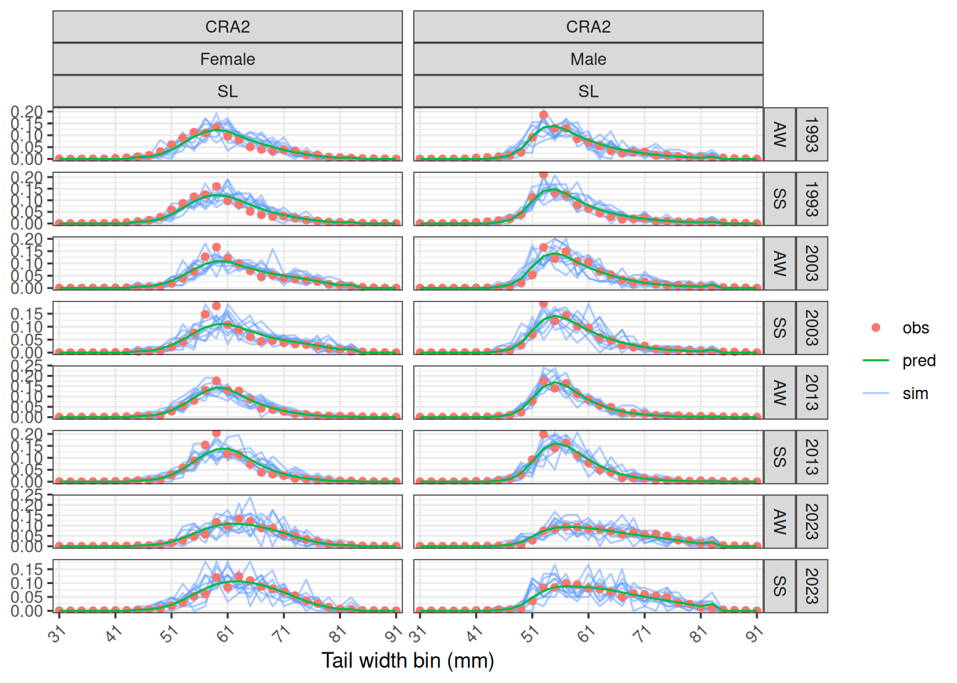
Calculate standard deviations of all model parameters, including non linear functions of random effects and parameters specified through the ADREPORT() macro from the user template. Check that the Hessian is positive definite. Try the analytical Hessian:
# Report <- sdreport(obj)
# print(Report$pdHess)
# he <- obj$he()
# he_inv <- solve(he)
# he_ch <- chol(he)
# ev <- eigen(he)
# range(ev$values)
Model weights
Francis length-frequency iterative re-weighting (Francis 2011).
names(tags)
#>  [1] "Event"         "Sex"           "RelMonth"      "RelYear"
#>  [5] "RecMonth"      "RecYear"       "DaysatLiberty" "gi_L1"
#>  [9] "gi_L2"         "TWConvertRel"  "TWConvertRec"  "TagRelease"
#> [13] "RelStatArea"   "Condition"     "Tagtype"       "RecStatArea"
#> [17] "gi_obs"        "gi_liberty"    "gi_sex"        "gi_morph"
plot_tag_residuals(data = data, obj = obj, type = "Pearson", xvar = "gi_L1")
#> # A tibble: 1 × 2
#>    SDNR   MAR
#>   <dbl> <dbl>
#> 1  1.02 0.620
#> [1] "SDNR should be close to 1 and MAR should be close to 0.67"
# plot_tag_residuals(data = data, obj = obj, type = "Pearson", xvar = "gi_liberty")
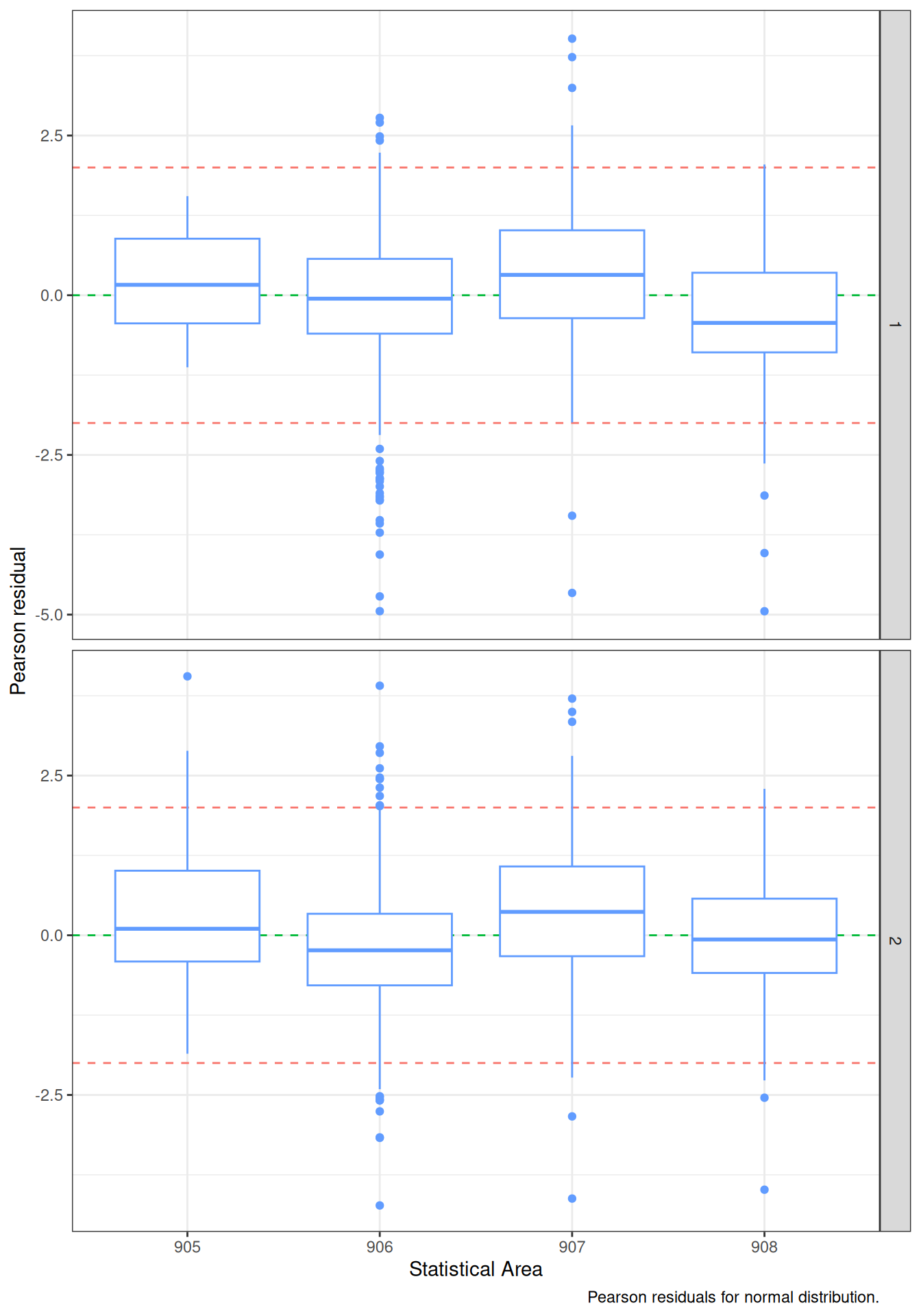
plot_tag_residuals(data = data, obj = obj, type = "Pearson", xvar = "RelStatArea")
#> # A tibble: 1 × 2
#>    SDNR   MAR
#>   <dbl> <dbl>
#> 1  1.02 0.620
#> [1] "SDNR should be close to 1 and MAR should be close to 0.67"
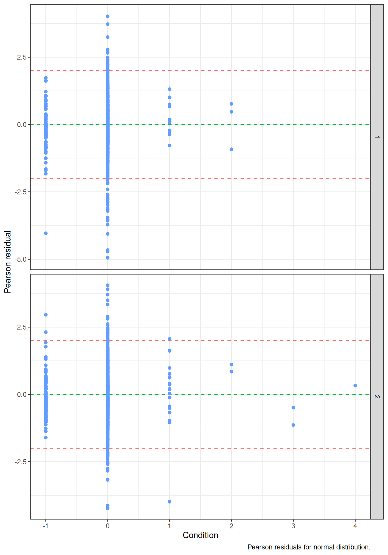
plot_tag_residuals(data = data, obj = obj, type = "Pearson", xvar = "Condition")
#> # A tibble: 1 × 2
#>    SDNR   MAR
#>   <dbl> <dbl>
#> 1  1.02 0.620
#> [1] "SDNR should be close to 1 and MAR should be close to 0.67"
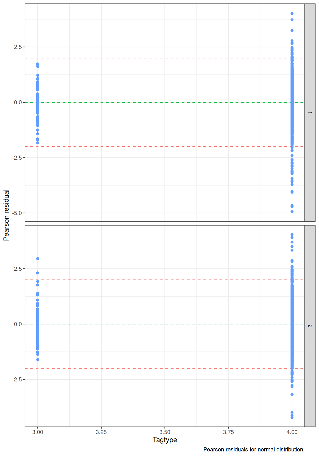
plot_tag_residuals(data = data, obj = obj, type = "Pearson", xvar = "Tagtype")
#> # A tibble: 1 × 2
#>    SDNR   MAR
#>   <dbl> <dbl>
#> 1  1.02 0.620
#> [1] "SDNR should be close to 1 and MAR should be close to 0.67"
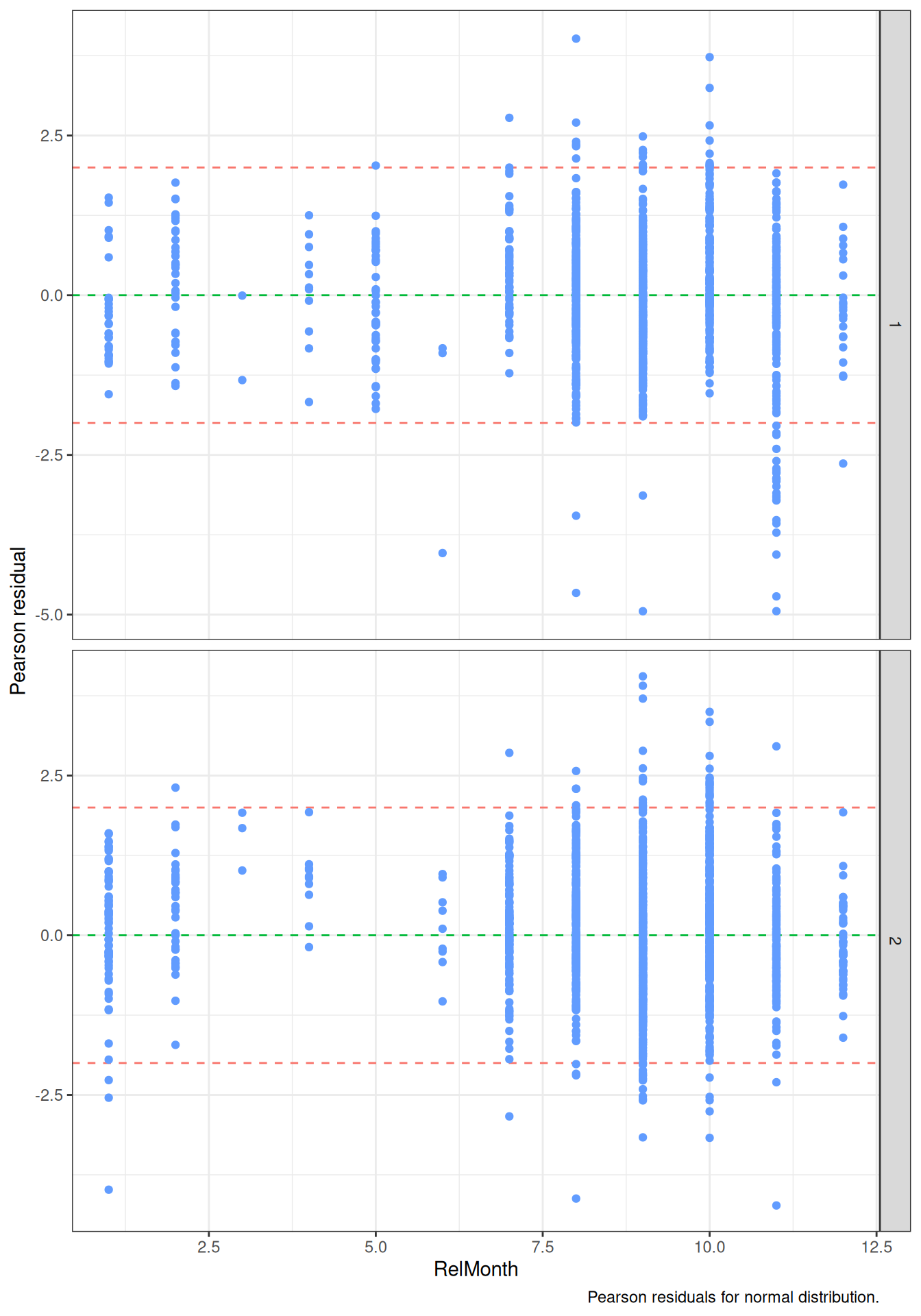
plot_tag_residuals(data = data, obj = obj, type = "Pearson", xvar = "RelMonth")
#> # A tibble: 1 × 2
#>    SDNR   MAR
#>   <dbl> <dbl>
#> 1  1.02 0.620
#> [1] "SDNR should be close to 1 and MAR should be close to 0.67"

get_lf_Francis(data = data, obj = obj)
#> # A tibble: 2 × 7
#> # Groups:   region, sex [2]
#>   region   sex    sd     n Francis_mult orig_wt new_wt
#>    <dbl> <dbl> <dbl> <int>        <dbl>   <dbl>  <dbl>
#> 1      1     1  1.21    62        0.696   1.20   0.838
#> 2      1     2  1.16    62        0.752   0.982  0.738
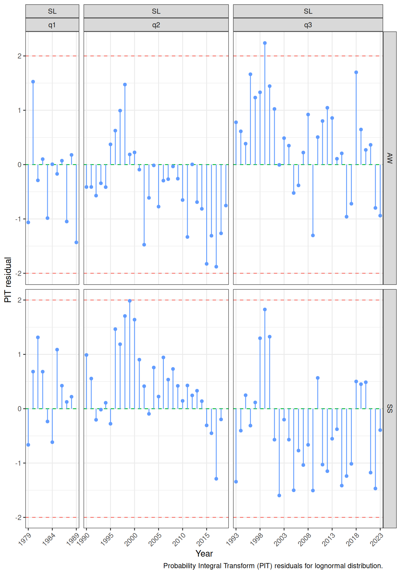
plot_cpue_residuals(data = data, obj = obj, type = "PIT")
#> # A tibble: 3 × 3
#>   q      SDNR   MAR
#>   <fct> <dbl> <dbl>
#> 1 q1    0.797 0.616
#> 2 q2    0.857 0.451
#> 3 q3    0.982 0.775
#> [1] "SDNR should be close to 1 and MAR should be close to 0.67"
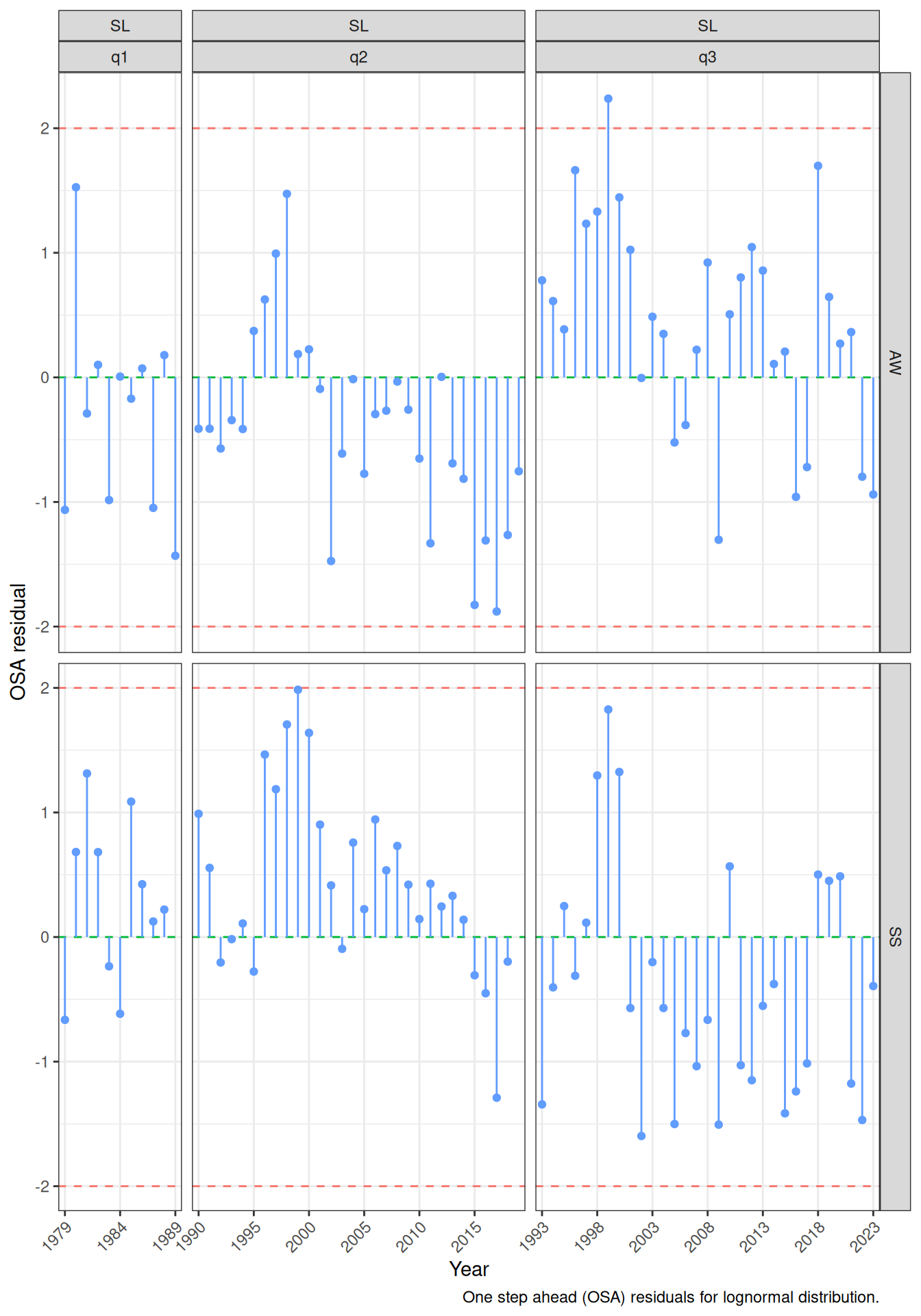
plot_cpue_residuals(data = data, obj = obj, type = "OSA")
#> # A tibble: 3 × 3
#>   q      SDNR   MAR
#>   <fct> <dbl> <dbl>
#> 1 q1    0.797 0.616
#> 2 q2    0.857 0.451
#> 3 q3    0.982 0.775
#> [1] "SDNR should be close to 1 and MAR should be close to 0.67"
plot_sexr_residuals(data = data, obj = obj, type = "PIT")
#>       SDNR       MAR
#> 1 1.074625 0.5652161
#> [1] "SDNR should be close to 1 and MAR should be close to 0.67"
# plot_sexr_residuals(data = data, obj = obj, type = "OSA")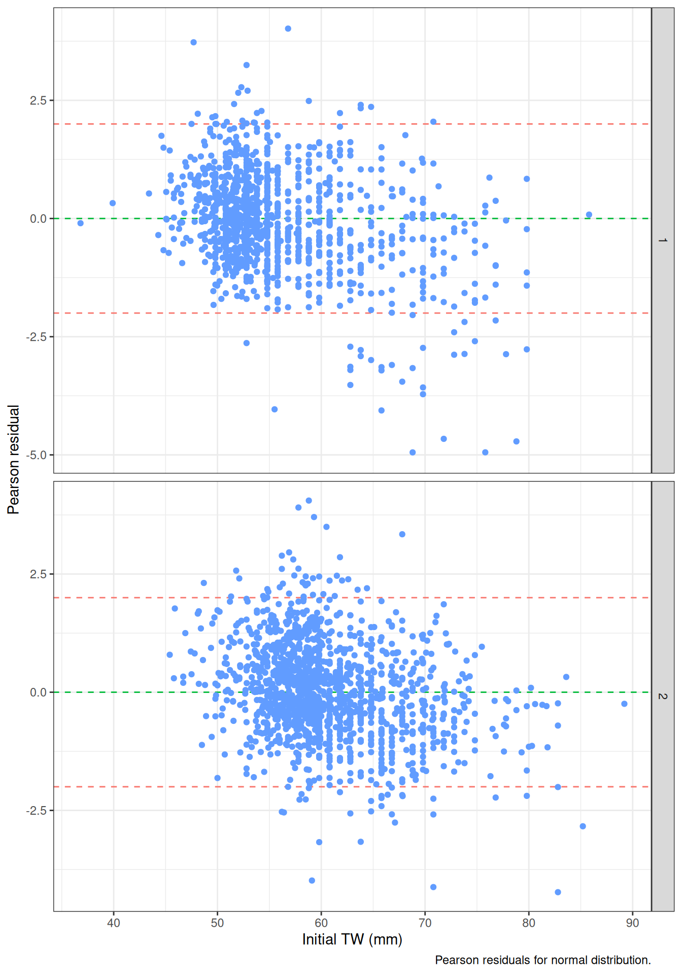
Model fits
plot_growth_increment(data = data, parameters = parameters, obj = obj, tau = 1)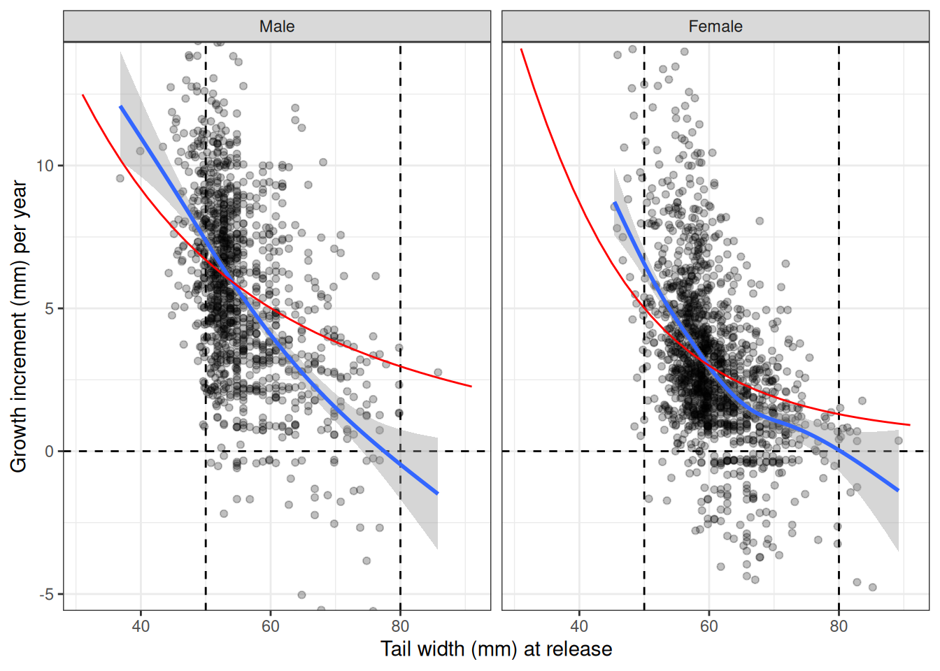
plot_growth_density(data = data, obj = obj)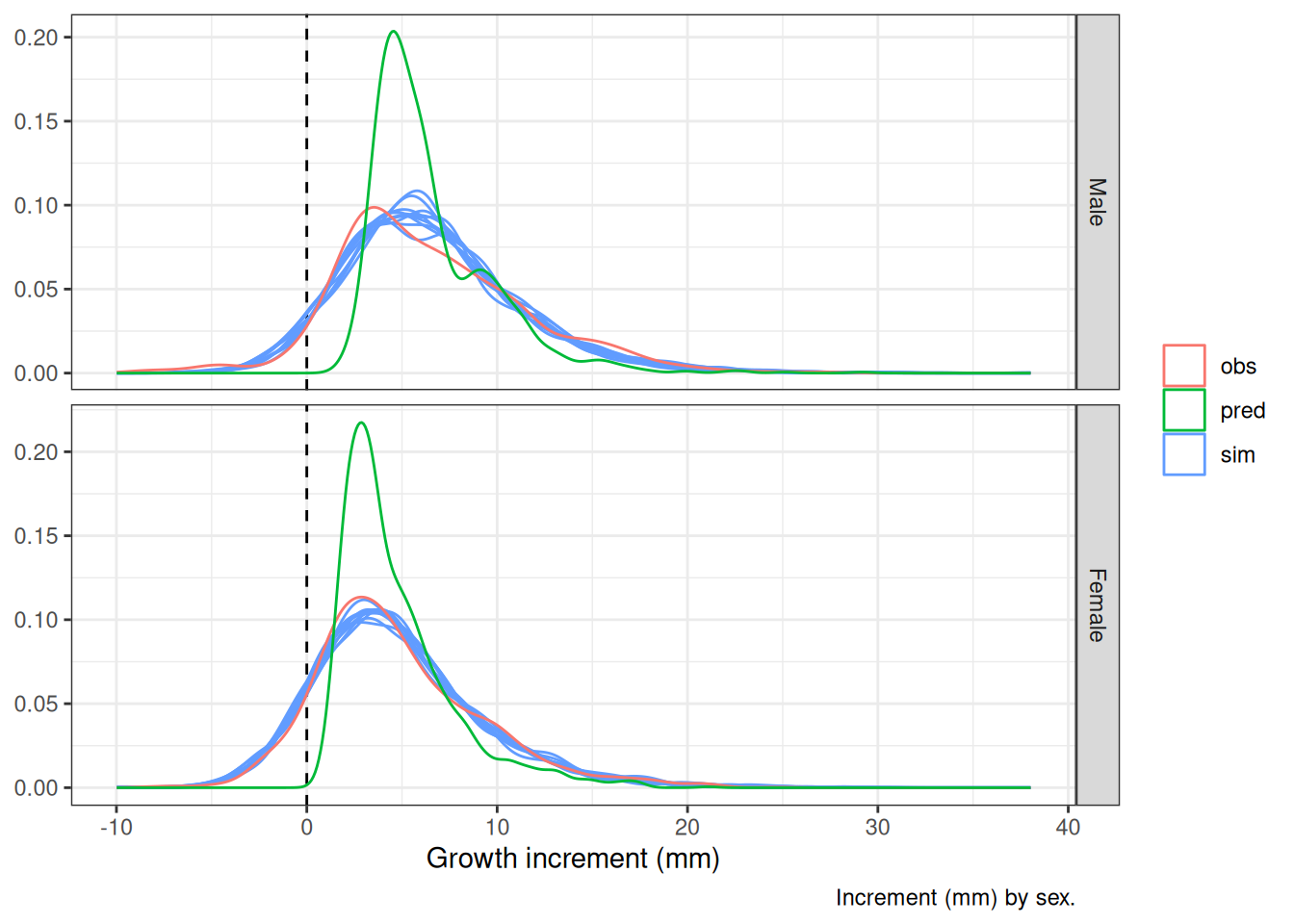
nsim <- 5
plot_catch(data = data, obj = obj, nsim = nsim)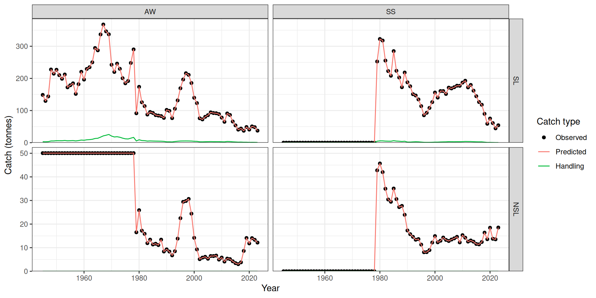
plot_catch_residuals(data = data, obj = obj)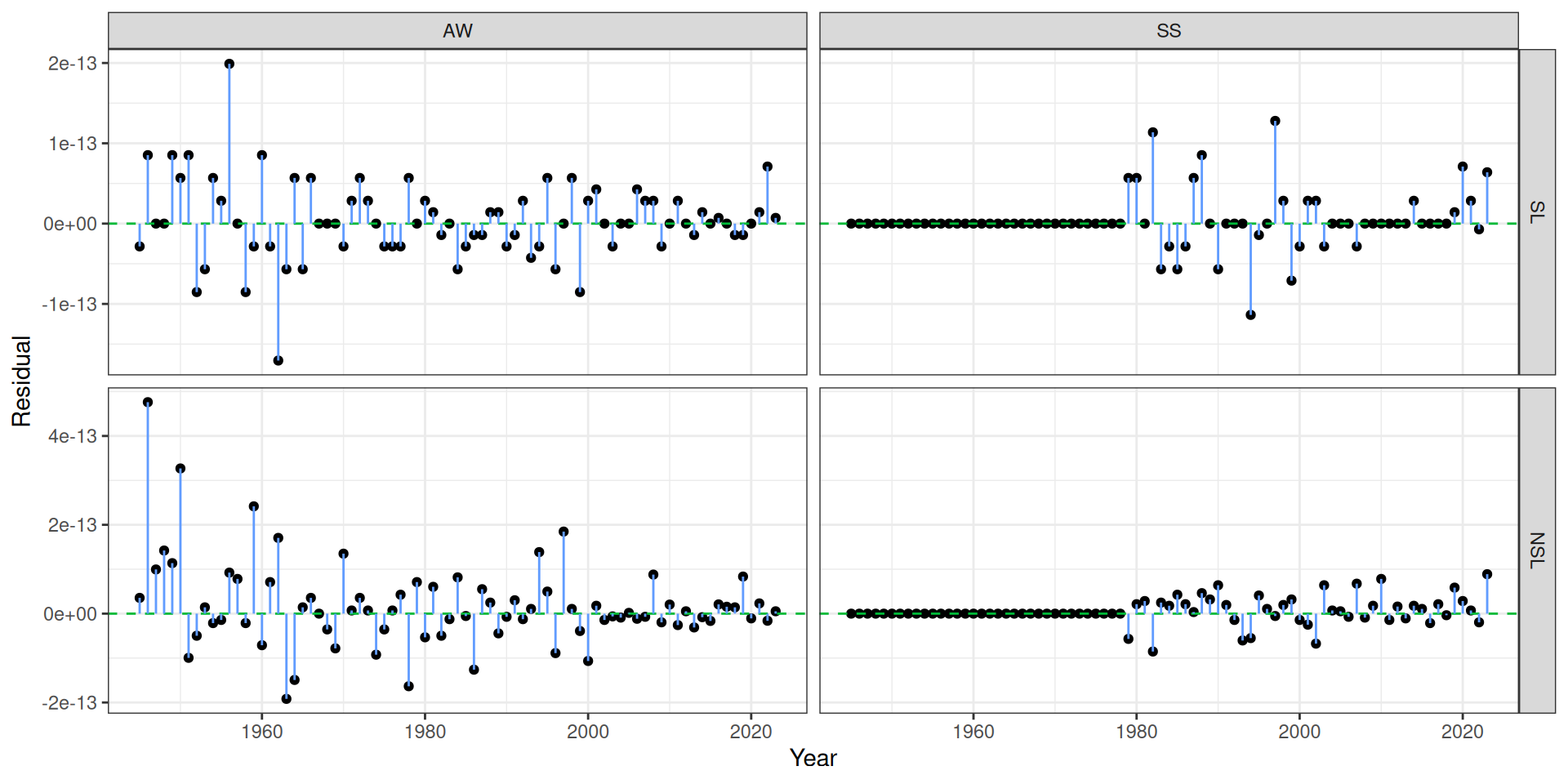
plot_cpue(data = data, obj = obj, nsim = nsim)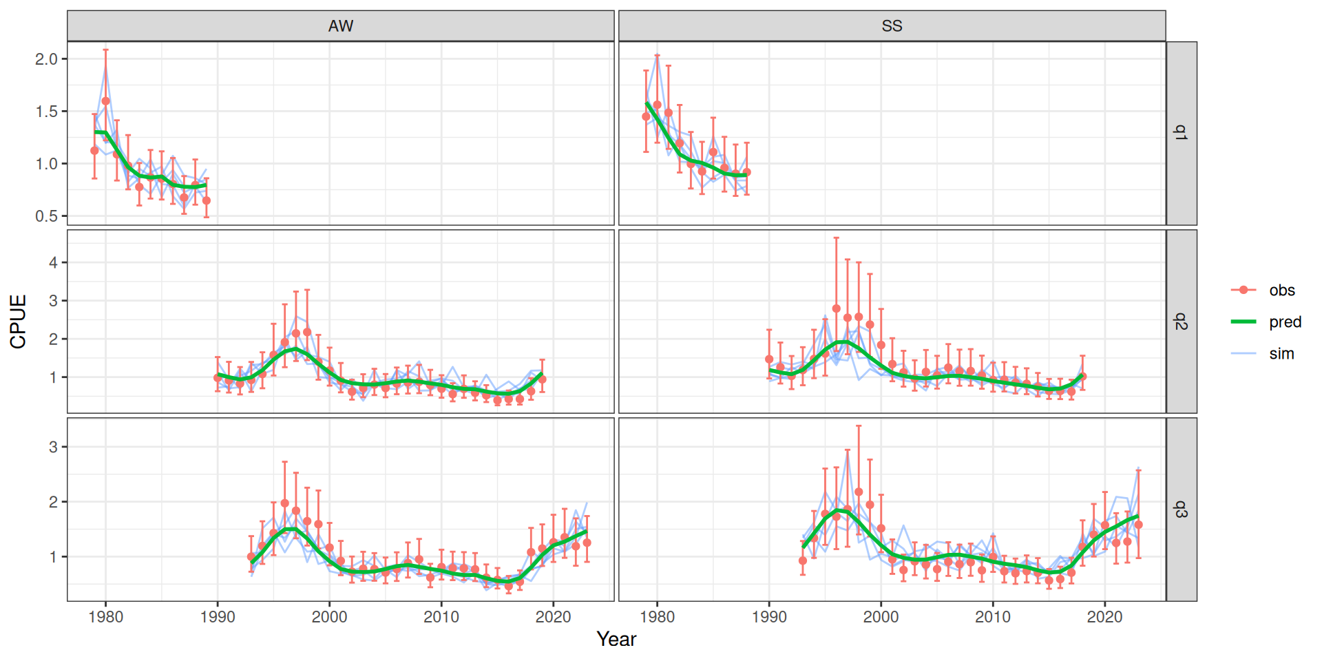
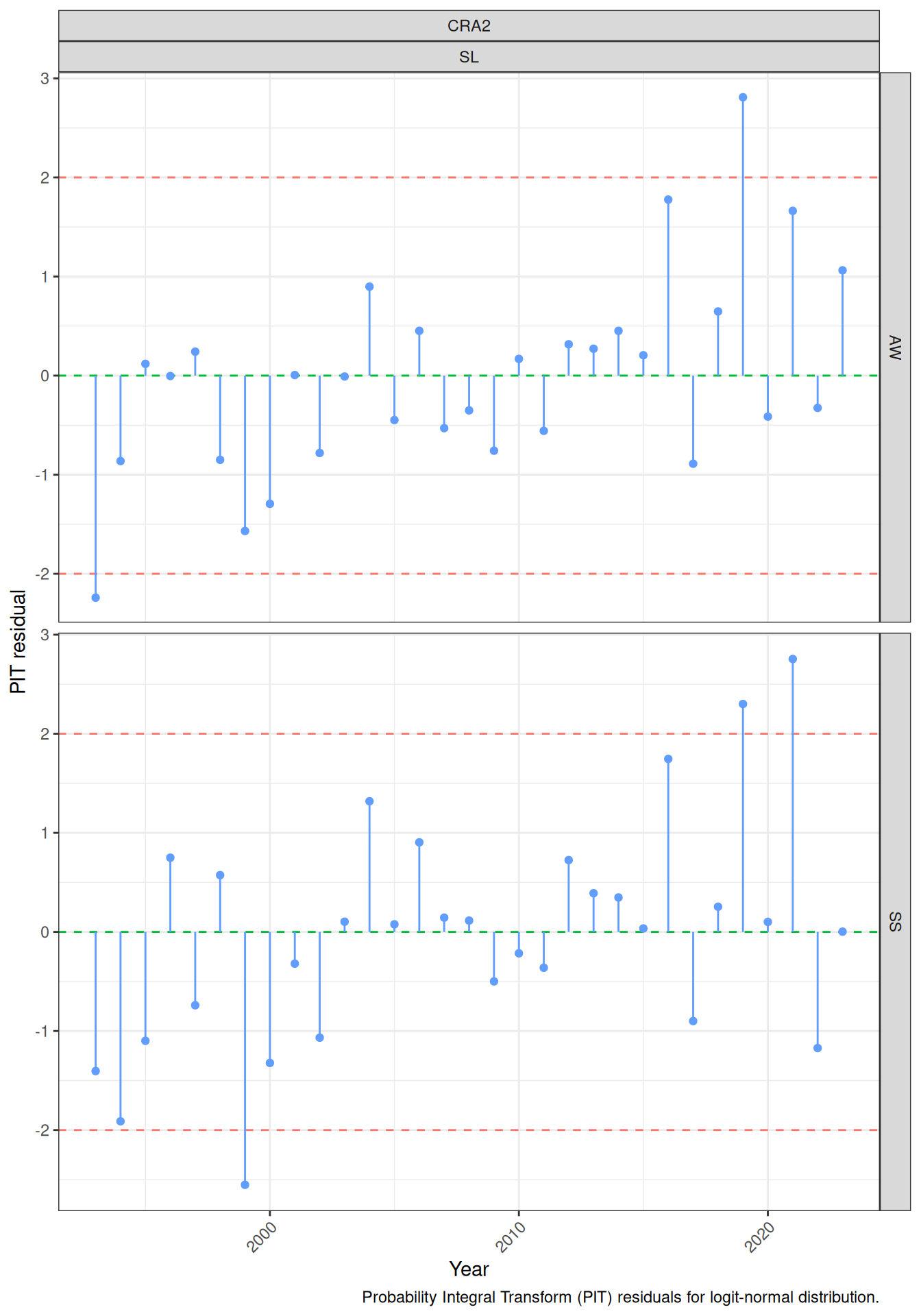
plot_cpue_residuals(data = data, obj = obj, type = "PIT")
#> # A tibble: 3 × 3
#>   q      SDNR   MAR
#>   <fct> <dbl> <dbl>
#> 1 q1    0.797 0.616
#> 2 q2    0.857 0.451
#> 3 q3    0.982 0.775
#> [1] "SDNR should be close to 1 and MAR should be close to 0.67"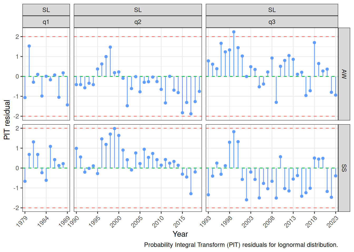
Ideally, Probability Integral Transform (PIT) residuals should appear as a roughly uniform distribution when plotted on a histogram, meaning the points should be scattered randomly around a horizontal line with no clear patterns, indicating that the model is accurately capturing the data’s probability distribution across different values of the response variable.
When plotted on a histogram, the distribution of PIT residuals should resemble a uniform distribution between 0 and 1, with no significant clustering at any particular point.
A scatter plot of PIT residuals against fitted values should not show any discernible patterns, like funneling or fanning, which would suggest issues with heteroscedasticity (unequal variance). Large deviations from the uniform distribution, especially at the extreme ends, could indicate potential outliers or model misspecification.
plot_sexr(data = data, obj = obj, nsim = 15)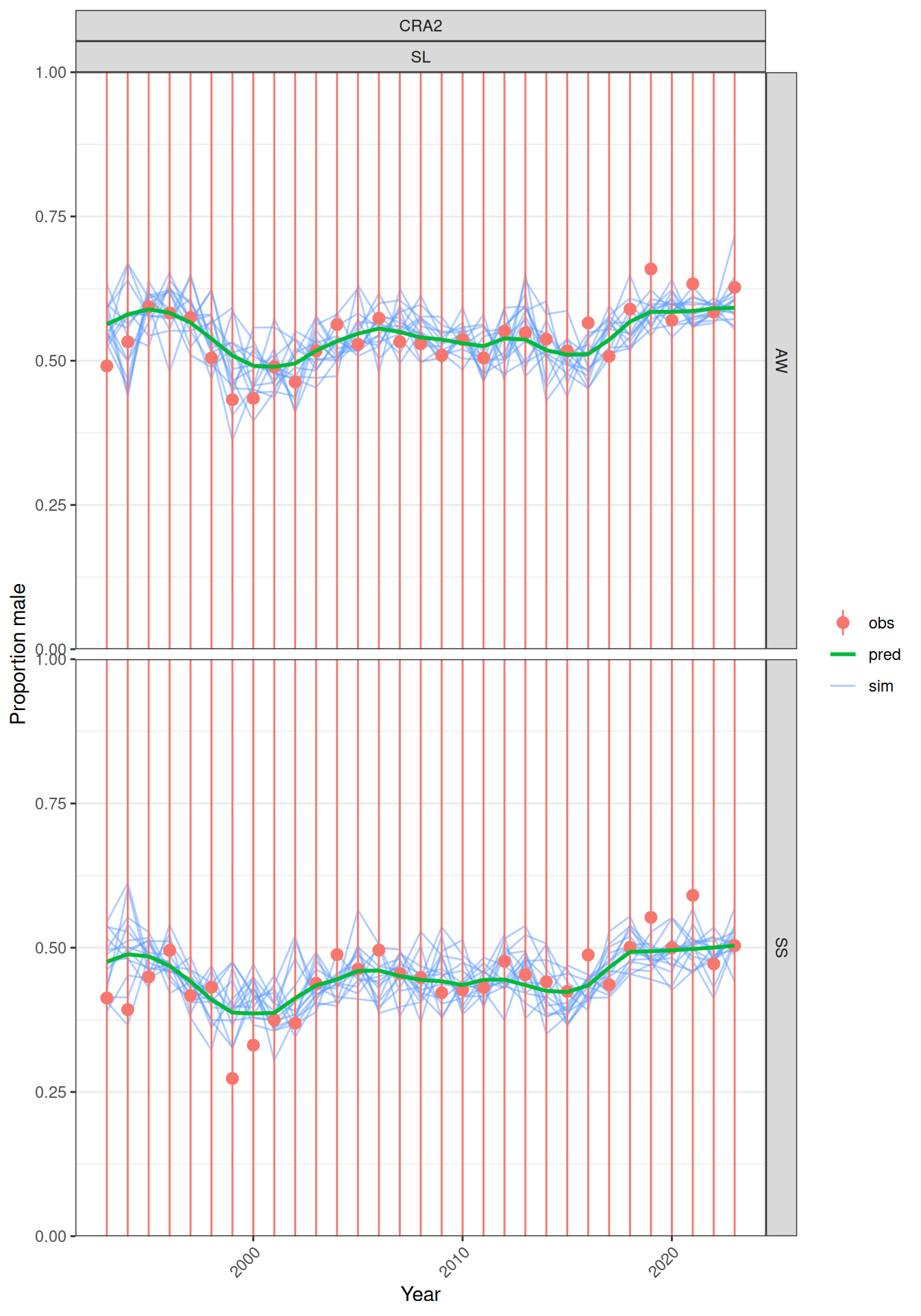
# plot_sexr_residuals(data = data, obj = obj, type = "Raw")
# plot_sexr_residuals(data = data, obj = obj, type = "old")
plot_sexr_residuals(data = data, obj = obj, type = "PIT")
#>       SDNR       MAR
#> 1 1.074625 0.5652161
#> [1] "SDNR should be close to 1 and MAR should be close to 0.67"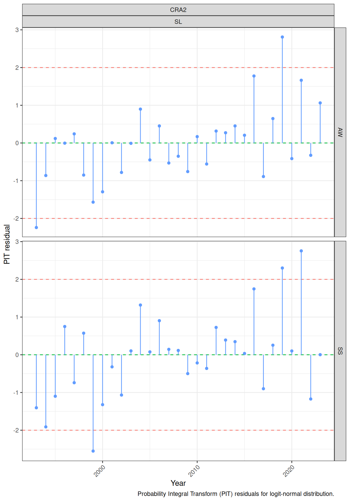
plot_lfs(data = data, obj = obj, nsim = nsim)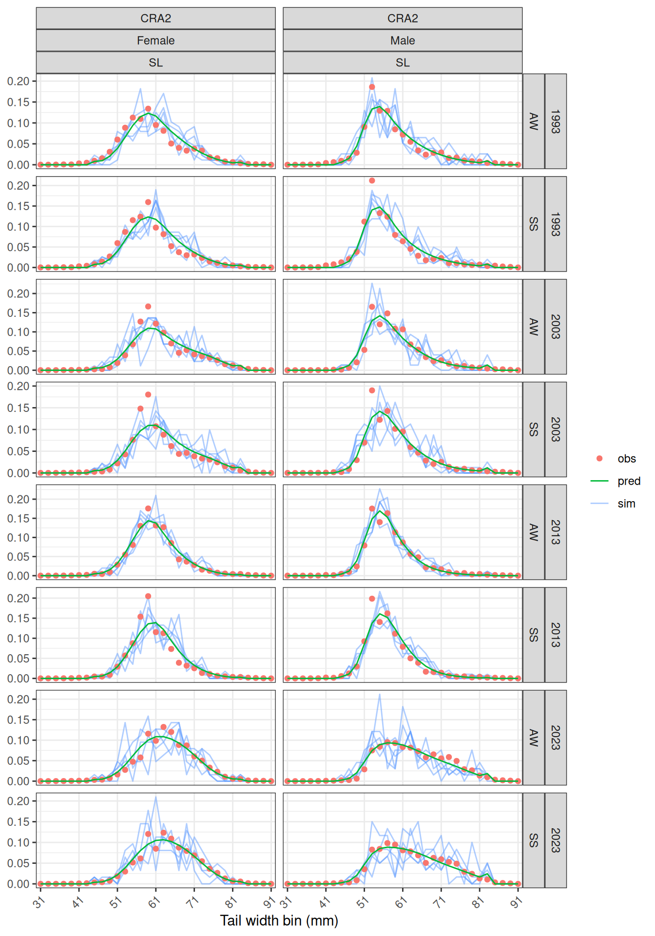
# plot_Fs(data = data, obj = obj)
plot_Us(data = data, obj = obj)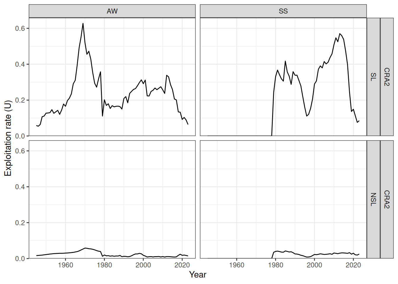
One step ahead residuals
Plot the one step ahead (OSA) residuals for the LFs using the R package compResidual (https://github.com/fishfollower/compResidual):
# TMB:::install.contrib("https://github.com/vtrijoulet/OSA_multivariate_dists/archive/main.zip")
# remotes::install_github("fishfollower/compResidual/compResidual", force=TRUE)
# library(compResidual)
# plot_lf_residuals(data = data, obj = obj, pick_one = 1)
# plot_lf_residuals(data = data, obj = obj, pick_one = 6)
# plot_lf_residuals(data = data, obj = obj, pick_one = 7)
# plot_lf_residuals(data = data, obj = obj, pick_one = 8)
osa_cpue <- oneStepPredict(obj = obj, observation.name = "cpue_obs")
#> [1] 142
#> [1] 141
#> [1] 140
#> [1] 139
#> [1] 138
#> [1] 137
#> [1] 136
#> [1] 135
#> [1] 134
#> [1] 133
#> [1] 132
#> [1] 131
#> [1] 130
#> [1] 129
#> [1] 128
#> [1] 127
#> [1] 126
#> [1] 125
#> [1] 124
#> [1] 123
#> [1] 122
#> [1] 121
#> [1] 120
#> [1] 119
#> [1] 118
#> [1] 117
#> [1] 116
#> [1] 115
#> [1] 114
#> [1] 113
#> [1] 112
#> [1] 111
#> [1] 110
#> [1] 109
#> [1] 108
#> [1] 107
#> [1] 106
#> [1] 105
#> [1] 104
#> [1] 103
#> [1] 102
#> [1] 101
#> [1] 100
#> [1] 99
#> [1] 98
#> [1] 97
#> [1] 96
#> [1] 95
#> [1] 94
#> [1] 93
#> [1] 92
#> [1] 91
#> [1] 90
#> [1] 89
#> [1] 88
#> [1] 87
#> [1] 86
#> [1] 85
#> [1] 84
#> [1] 83
#> [1] 82
#> [1] 81
#> [1] 80
#> [1] 79
#> [1] 78
#> [1] 77
#> [1] 76
#> [1] 75
#> [1] 74
#> [1] 73
#> [1] 72
#> [1] 71
#> [1] 70
#> [1] 69
#> [1] 68
#> [1] 67
#> [1] 66
#> [1] 65
#> [1] 64
#> [1] 63
#> [1] 62
#> [1] 61
#> [1] 60
#> [1] 59
#> [1] 58
#> [1] 57
#> [1] 56
#> [1] 55
#> [1] 54
#> [1] 53
#> [1] 52
#> [1] 51
#> [1] 50
#> [1] 49
#> [1] 48
#> [1] 47
#> [1] 46
#> [1] 45
#> [1] 44
#> [1] 43
#> [1] 42
#> [1] 41
#> [1] 40
#> [1] 39
#> [1] 38
#> [1] 37
#> [1] 36
#> [1] 35
#> [1] 34
#> [1] 33
#> [1] 32
#> [1] 31
#> [1] 30
#> [1] 29
#> [1] 28
#> [1] 27
#> [1] 26
#> [1] 25
#> [1] 24
#> [1] 23
#> [1] 22
#> [1] 21
#> [1] 20
#> [1] 19
#> [1] 18
#> [1] 17
#> [1] 16
#> [1] 15
#> [1] 14
#> [1] 13
#> [1] 12
#> [1] 11
#> [1] 10
#> [1] 9
#> [1] 8
#> [1] 7
#> [1] 6
#> [1] 5
#> [1] 4
#> [1] 3
#> [1] 2
#> [1] 1
dim(osa_cpue)
#> [1] 142   5
length(data$cpue_obs)
#> [1] 142
plot_cpue_residuals(data = data, obj = obj, type = "PIT")
#> # A tibble: 3 × 3
#>   q      SDNR   MAR
#>   <fct> <dbl> <dbl>
#> 1 q1    0.797 0.616
#> 2 q2    0.857 0.451
#> 3 q3    0.982 0.775
#> [1] "SDNR should be close to 1 and MAR should be close to 0.67"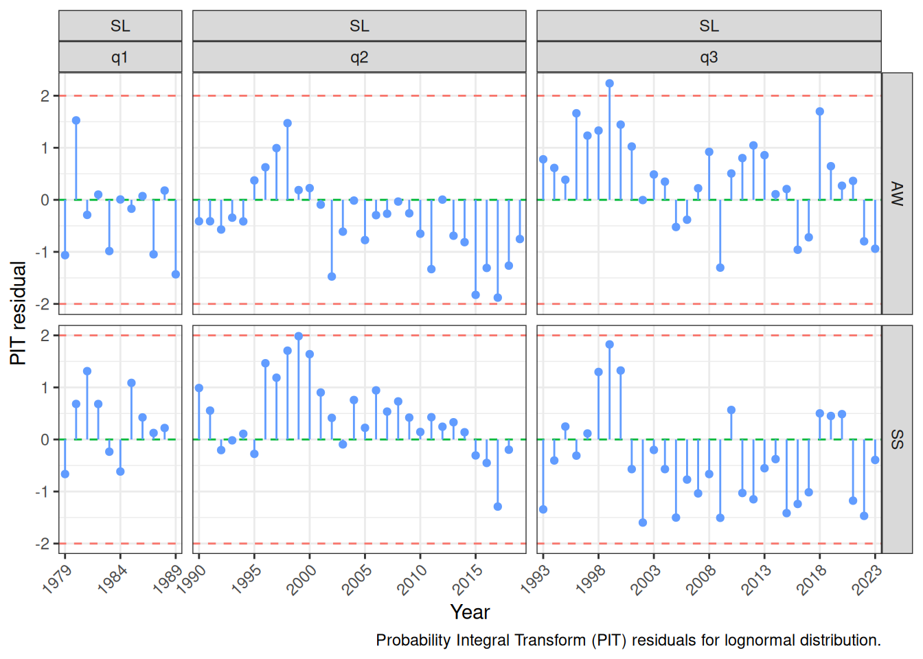
plot_cpue_residuals(data = data, obj = obj, type = "OSA")
#> # A tibble: 3 × 3
#>   q      SDNR   MAR
#>   <fct> <dbl> <dbl>
#> 1 q1    0.797 0.616
#> 2 q2    0.857 0.451
#> 3 q3    0.982 0.775
#> [1] "SDNR should be close to 1 and MAR should be close to 0.67"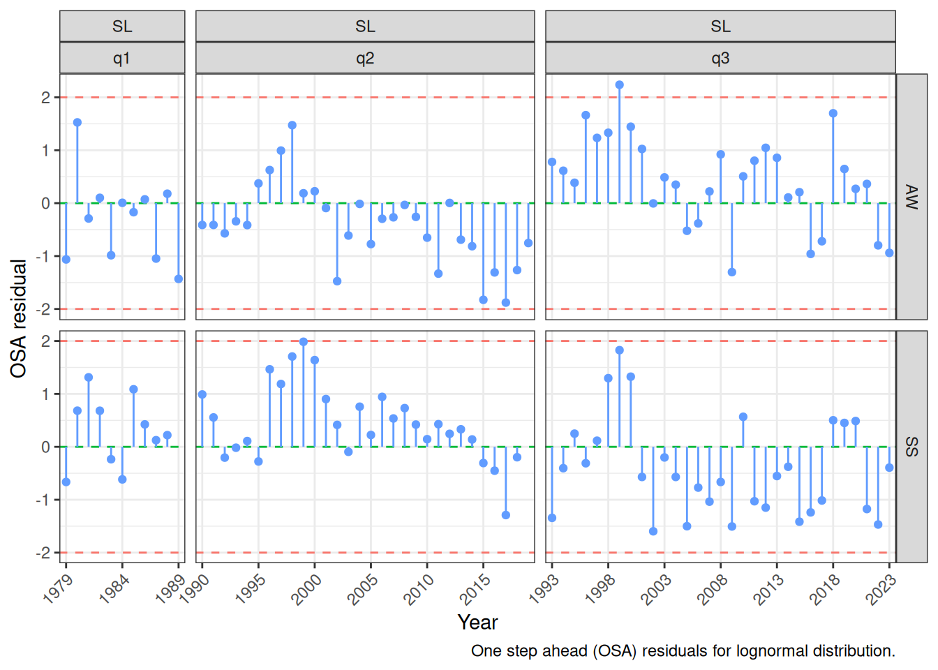
Projections
# i1 <- which(c(first_year:last_year) == 1979)
# i1 <- which(c(first_year:last_year) == min(lf$fyear))
# i1 <- 1
# sim <- project_recruitment(object = obj, h = 5, y1 = NULL, y2 = NULL)
#
# library(forecast)
# i1 <- which(c(first_year:last_year) == 1979)
# i1 <- which(c(first_year:last_year) == min(lf$fyear))
# i1 <- 1
# Rdevs <- obj$report(obj$env$last.par.best)$Rdev_yr[i1:n_year,1]
# fit <- auto.arima(y = Rdevs, max.p = 0, max.d = 5, max.q = 5, approximation = FALSE, stepwise = FALSE, ic = "bic", trace = TRUE)
# fit <- auto.arima(y = Rdevs, max.p = 5, max.d = 0, max.q = 5, approximation = FALSE, stepwise = FALSE, ic = "bic", trace = TRUE)
# fit <- auto.arima(y = Rdevs, max.p = 5, max.d = 5, max.q = 0, approximation = FALSE, stepwise = FALSE, ic = "bic", trace = TRUE)
# fit <- auto.arima(y = Rdevs, approximation = FALSE, stepwise = FALSE, ic = "bic", trace = TRUE)
# checkresiduals(fit)
# autoplot(fit)
# autoplot(forecast(fit, h = 5))
# autoplot(simulate(object = fit, nsim = 5, future = TRUE, bootstrap = TRUE))
#
# fc <- forecast(object = fit, h = 5)
#
# df1 <- data.frame(x = 1:length(Rdevs), mean = Rdevs, group = 1)
# df2 <- data.frame(x = 80:84, mean = fc$mean, lower = fc$lower, upper = fc$upper, group = 2)
# df <- bind_rows(df1, df2)
#
# p <- ggplot(data = df, aes(x = x, y = mean, group = group)) +
#   geom_ribbon(aes(ymin = lower.95., ymax = upper.95.), alpha = 0.5, color = NA, fill = "lightblue") +
#   geom_ribbon(aes(ymin = lower.80., ymax = upper.80.), alpha = 0.5, color = NA, fill = "blue") +
#   geom_line(color = "blue")
#
# for (i in 1:10) {
#   sim <- simulate(object = fit, nsim = 5, future = TRUE, bootstrap = TRUE)
#   dsim <- data.frame(x = 80:84, mean = sim, group = 3)
#   p <- p + geom_line(data = dsim, size = 0.3)
# }
#
# p
A likelihood profile (Hilborn and Walters 1992) for log_Ma can be done using:
# prof <- TMB::tmbprofile(obj = obj, name = "Rdev_yr[65,1]")
# lincomb <- as.numeric(names(obj$par) == "log_Ma")
# prof <- TMB::tmbprofile(obj = obj, lincomb = lincomb)
# plot(prof)
# confint(prof)
# df <- likelihood_profile(obj = obj, name = "log_Ma")
# lincomb <- rep(0, length(obj$par))
# names(obj$par)
# names(obj$par)[68]
# lincomb[68] <- 1
# prof_mle <- tmbprofile2(obj = obj, lincomb = lincomb)
# # prof_mcmc <- get_mcmc_profile(obj = obj, mcmc = mcmc1, name = "log_galpha[1]")
# names(obj$par)[names(obj$par) == "Rdev_yr"]
# prof_mcmc <- get_mcmc_profile(obj = obj, mcmc = mcmc1, name = "Rdev_yr[42]")
#
# plot_profile(x = prof_mle, lab = "log(Galpha)")
# ggsave(file = "like_prof1.png", width = 9)
# plot_profile(x = prof_mle, y = prof_mcmc, lab = "log(M)", rescale = FALSE)
# ggsave(file = "like_prof2.png", width = 9)
# plot_profile(x = prof_mle, y = prof_mcmc, lab = "log(M)")
# ggsave(file = "like_prof3.png", width = 9)
#
# prof_mle <- tmbprofile2(obj = obj, name = "log_Ma")
# prof_mcmc <- get_mcmc_profile(obj = obj, mcmc = mcmc1, name = "log_Ma")
#
# plot_profile(x = prof_mle, lab = "log(M)")
# ggsave(file = "like_prof1.png", width = 9)
# plot_profile(x = prof_mle, y = prof_mcmc, lab = "log(M)", rescale = FALSE)
# ggsave(file = "like_prof2.png", width = 9)
# plot_profile(x = prof_mle, y = prof_mcmc, lab = "log(M)")
# ggsave(file = "like_prof3.png", width = 9)
Fournier, David, and C. P. Archibald. 1982. “A General Theory for Analyzing Catch at Age Data.” Canadian Journal of Fisheries and Aquatic Sciences 39 (8): 1195–207. https://doi.org/10.1139/f82-157.
Francis, R. I. C. Chris. 2011. “Data Weighting in Statistical Fisheries Stock Assessment Models.” Canadian Journal of Fisheries and Aquatic Sciences 68 (6): 1124–38. https://doi.org/10.1139/f2011-025.
Hilborn, Ray, and Carl J. Walters. 1992. Quantitative Fisheries Stock Assessment: Choice, Dynamics and Uncertainty. Chapman; Hall. https://doi.org/10.1007/978-1-4615-3598-0.
Kristensen, Kasper, Anders Nielsen, Casper W. Berg, Hans Skaug, and Bradley M. Bell. 2016. “TMB: Automatic Differentiation and Laplace Approximation.” Journal of Statistical Software 70 (5): 1–21. https://doi.org/10.18637/jss.v070.i05.
Maunder, Mark N., and André E. Punt. 2004. “Standardizing Catch and Effort Data: A Review of Recent Approaches.” Fisheries Research 70 (2–3): 141–59. https://doi.org/10.1016/j.fishres.2004.08.002.
Quinn, Terrance J., and Richard B. Deriso. 1999. Quantitative Fish Dynamics. Oxford University Press.
Schnute, Jon, and David Fournier. 1980. “A New Approach to Estimating Populations and Stock Composition in Mark-Recapture Experiments.” Canadian Journal of Fisheries and Aquatic Sciences 37 (10): 1744–59. https://doi.org/10.1139/f80-220.
Webber, Darcy N., and Jeremy R. McKenzie. 2022. Rock Lobster (CRA 2) Stock Assessment for the 2021-22 Fishing Year. 2022/XX. New Zealand Fisheries Stock Assessment Report.
Webber, Darcy N., and Jeremy R. McKenzie. 2024. Rock Lobster (CRA 2) Stock Assessment for the 2023-24 Fishing Year. 2024/XX. New Zealand Fisheries Assessment Report.