
# remotes::install_github("noaa-afsc/SparseNUTS")
if (dir.exists(file.path("..", "R")) && requireNamespace("pkgload", quietly = TRUE)) {
  pkgload::load_all("..", quiet = TRUE)
} else {
  library(decamod)
}
library(TMBhelper)
library(tidyverse)
library(kableExtra)
library(SparseNUTS)

theme_set(theme_bw())

options(mc.cores = parallel::detectCores() - 1) # Specify the number of coresThe surplus production model (SPM) is a state-space implementation of the Schaefer surplus production model (Schaefer 1954). The model is described in detail in the decamod package documentation. Here, we provide an example of how to fit the SPM to catch and CPUE data using TMB and the adnuts package for Bayesian inference.
where is the observed catch and is the surplus production defined as:
where is the carrying capacity, is the intrinsic growth rate, and is a shape parameter. When , the model reduces to the Schaefer model (Schaefer 1954). More general formulations, including the Pella-Tomlinson model, allow for asymmetric surplus production (Hilborn and Walters 1992; Quinn and Deriso 1999).
Load inputs
Define model
Define the data list.
catch <- read_csv(system.file("extdata", "CRA2_catch_data_input.csv", package = "decamod")) %>%
# catch <- read_csv("CRA2_catch_data_input.csv") %>%
# catch <- catch_CRA2 %>%
  filter(Year > 1978) %>%
  mutate(TotalCatch = Commercial + Recreational + Illegal + Customary) %>%
  select(Year, Season, Catch = TotalCatch) %>%
  arrange(Year, Season) %>%
  mutate(Period = 1:n())

ys <- catch %>%
  # mutate(Year = as.character(Year)) %>%
  select(Year, Season, Period)

logbook_CRA2 <- read_csv(system.file("extdata", "CRA2_LB_CPUE_legal_2025.csv", package = "decamod"))

cpue <- bind_rows(
  fsu_CRA2 %>% mutate(Index = "FSU"),
  celr_CRA2 %>% mutate(Index = "CELR"),
  logbook_CRA2 %>% mutate(Index = "Logbook")
  ) %>%
  filter(Year > 1978) %>%
  separate(Year, into = c("Year", "season"), sep = "_") %>%
  mutate(Year = as.numeric(Year), Season = ifelse(season == "AW", 1, 2)) %>%
  # mutate(Year = as.character(Year)) %>%
  mutate(q = case_when(
    Index == "FSU" & season == "AW" ~ 1,
    Index == "FSU" & season == "SS" ~ 2,
    Index == "CELR" & season == "AW" ~ 3,
    Index == "CELR" & season == "SS" ~ 4,
    Index == "Logbook" & season == "AW" ~ 5,
    Index == "Logbook" & season == "SS" ~ 6
  )) %>%
  mutate(logSD = log(1 + SD / Mean)) %>%
  left_join(ys, by = join_by(Year, Season)) %>%
  select(Year, Season, Period, Median, logSD, q, Index)

data <- list(
  n_time = nrow(catch),
  catch_time = catch$Period,
  catch_season = catch$Season,
  catch_obs = catch$Catch,
  cpue_time = cpue$Period,
  cpue_season = cpue$Season,
  cpue_q = cpue$q,
  cpue_obs = cpue$Median,
  cpue_sd = cpue$logSD
)

n_q <- length(unique(cpue$q))
n_time <- max(data$catch_time)
Define the parameters list.
parameters <- list(
  log_r = log(0.35),
  log_z = log(1),
  log_K = log(5000),
  logit_D0 = qlogis(0.5),   # logit ensures 0 < D0 < 1, qlogis accepts values up to 0.999999
  log_q = log(rep(0.001, n_q)),
  log_cpue_pow = log(1),
  log_cpue_pro = log(rep(1e-6, n_q)),
  cpue_creep = 0.01, # proportional linear increase per observation within each CPUE series
  log_sigmap = log(0.001),
  log_B = log(rep(2000, n_time - 1))
  # epsilon = rep(0, n_time)
)
priors <- list()
priors[["log_r"]] <- list(type = "normal", par1 = log(0.35), par2 = 0.5, index = which("log_r" == names(parameters)))
priors[["log_z"]] <- list(type = "normal", par1 = 0, par2 = 0.1, index = which("log_z" == names(parameters)))
priors[["log_K"]] <- list(type = "normal", par1 = log(1000), par2 = 1, index = which("log_K" == names(parameters)))
priors[["logit_D0"]] <- list(type = "normal", par1 = qlogis(0.5), par2 = 0.5, index = which("logit_D0" == names(parameters)))
priors[["log_q"]] <- list(type = "normal", par1 = -5, par2 = 2, index = which("log_q" == names(parameters)))
priors[["log_cpue_pow"]] <- list(type = "normal", par1 = 0, par2 = 0.5, index = which("log_cpue_pow" == names(parameters)))
priors[["log_cpue_pro"]] <- list(type = "normal", par1 = 0, par2 = 0.5, index = which("log_cpue_pro" == names(parameters)))
priors[["log_sigmap"]] <- list(type = "normal", par1 = 0, par2 = 0.5, index = which("log_sigmap" == names(parameters)))
evaluate_priors(parameters, priors)
#> [1] -2401.345
# plot_priors(priors, bounds)
data$priors <- priorsCreate the AD object using the MakeADFun function from the TMB framework (Kristensen et al. 2016).
# obj <- MakeADFun(func = cmb(spm_model, data), parameters = parameters, map = map, random = "epsilon")
# obj <- MakeADFun(func = cmb(spm_model2, data), parameters = parameters, map = map, random = "log_B")
obj <- MakeADFun(func = cmb(spm_model, data), parameters = parameters, map = map, random = "log_B")
obj$simulate(par = obj$par)$cpue_obs
#>   [1]  2.880766  2.723061  3.285210  3.175249  3.417530  3.762678  3.961984
#>   [8]  3.855735  3.582760  3.500536  4.074791  4.397285  4.539514  4.463934
#>  [15]  4.567578  5.394497  4.357325  5.050792  4.300161  4.623374  4.823842
#>  [22]  4.138987  5.174022  4.861718  3.787004  5.751450  5.508774  4.578351
#>  [29]  4.731531  4.809274  4.995917  3.930471  3.929439  5.697597  4.891402
#>  [36]  5.364629  4.055185  4.442641  4.374508  4.621628  6.473469  5.599138
#>  [43]  5.602210  5.228421  5.613344  4.318656  5.334720  4.776136  4.691118
#>  [50]  3.442707  4.233411  4.308397  5.973751  3.868399  4.417564  4.019626
#>  [57]  5.262440  4.953658  5.872046  5.603603  6.725721  5.930084  4.844085
#>  [64]  6.029421  5.553198  4.563280  5.006434  5.705805  6.382971  5.282989
#>  [71]  6.323884  6.140580  7.156836  6.862526  5.781832  8.148995  5.530297
#>  [78]  6.115141  5.284246  5.340768  4.702933  4.026943  4.498813  5.111539
#>  [85]  4.091804  4.471509  4.210805  3.577132  5.249740  4.134323  5.010404
#>  [92]  5.129972  4.339118  4.804370  5.545025  4.617721  3.621442  6.023434
#>  [99]  4.531929  4.760994  6.681516  5.360170  5.065885  4.570049  6.920274
#> [106]  4.766386  4.904408  4.550228  5.321921  5.145371  5.101560  4.438760
#> [113]  4.838104  5.240897  6.189958  3.812971  6.332972  6.543727  4.871658
#> [120]  5.330500  5.842127  4.236831  4.506169  7.634649  4.150160  6.012713
#> [127]  5.031434  6.409105  6.485751  5.650683  5.891495  6.579010  4.944903
#> [134]  6.069478  4.998383  6.153063  5.719858  6.506556  6.964148 10.070518
#> [141]  5.833396  5.967020  7.362769  5.718512
List of parameters that are on:
Define parameter bounds.
Lwr <- rep(-Inf, length(obj$par))
Upr <- rep(Inf, length(obj$par))
Lwr[grep("log_r", names(obj$par))] <- -10
Upr[grep("log_r", names(obj$par))] <- 10
Lwr[grep("log_z", names(obj$par))] <- log(0)
Upr[grep("log_z", names(obj$par))] <- log(2)
Lwr[grep("log_K", names(obj$par))] <- log(300)
Upr[grep("log_K", names(obj$par))] <- log(300000)
Lwr[grep("logit_D0", names(obj$par))] <- qlogis(0.3)
Upr[grep("logit_D0", names(obj$par))] <- qlogis(0.7)
Lwr[grep("log_cpue_pow", names(obj$par))] <- log(0)
Upr[grep("log_cpue_pow", names(obj$par))] <- log(2)
Lwr[grep("log_q", names(obj$par))] <- -25
Upr[grep("log_q", names(obj$par))] <- 1
Lwr[grep("log_sigmap", names(obj$par))] <- log(0)
Upr[grep("log_sigmap", names(obj$par))] <- log(0.5)
Lwr[grep("log_cpue_pro", names(obj$par))] <- log(0)
Upr[grep("log_cpue_pro", names(obj$par))] <- log(2)

bounds <- data.frame(lower = Lwr, upper = Upr)
tibble(Parameter = names(obj$par), LB = Lwr, Initial = obj$par, UB = Upr)
#> # A tibble: 11 × 4
#>    Parameter        LB Initial     UB
#>    <chr>         <dbl>   <dbl>  <dbl>
#>  1 log_r       -10       -1.05 10
#>  2 log_z      -Inf        0     0.693
#>  3 log_K         5.70     8.52 12.6
#>  4 logit_D0     -0.847    0     0.847
#>  5 log_q       -25       -6.91  1
#>  6 log_q       -25       -6.91  1
#>  7 log_q       -25       -6.91  1
#>  8 log_q       -25       -6.91  1
#>  9 log_q       -25       -6.91  1
#> 10 log_q       -25       -6.91  1
#> 11 log_sigmap -Inf       -6.91 -0.693
Optimise using the nlminb function:
control <- list(eval.max = 100000, iter.max = 100000)
opt <- nlminb(start = obj$par, objective = obj$fn, gradient = obj$gr,
              control = control, lower = bounds$lower, upper = bounds$upper)
opt <- nlminb(start = opt$par, objective = obj$fn, gradient = obj$gr,
              control = control, lower = bounds$lower, upper = bounds$upper)
obj$par <- opt$par
obj$env$last.par <- opt$par
obj$env$last.par.best <- opt$par
report <- obj$report(obj$env$last.par.best)
# check_estimability(obj = obj)
tibble(par = names(obj$env$last.par.best), val = exp(obj$env$last.par.best))
#> # A tibble: 11 × 2
#>    par                val
#>    <chr>            <dbl>
#>  1 log_r         0.261
#>  2 log_z         0.988
#>  3 log_K      2449.
#>  4 logit_D0      1.73
#>  5 log_q         0.000725
#>  6 log_q         0.000853
#>  7 log_q         0.000839
#>  8 log_q         0.00114
#>  9 log_q         0.000827
#> 10 log_q         0.00109
#> 11 log_sigmap    0.126
# tibble(par = names(obj$par), val = obj$env$last.par.best, gr = obj$gr()) %>%
#   arrange(-gr)
# check_estimability(obj = obj)
biomass_df <- data.frame(Year = catch$Year, Season = catch$Season,
                         Pred = report$B,
                         Expected = report$Bmu) %>%
  mutate(Season = ifelse(Season == 1, "AW", "SS"))

set.seed(123)
sim_df <- NULL
for (i in 1:100) {
  df <- data.frame(Year = catch$Year, Season = catch$Season,
                   Sim = c(NA, exp(obj$simulate(par = obj$env$last.par.best)$log_B)),
                   iter = i)
  sim_df <- bind_rows(sim_df, df)
}
sim_df <- sim_df %>%
  mutate(Season = ifelse(Season == 1, "AW", "SS"))

ggplot(data = biomass_df, aes(x = as.numeric(Year), y = Pred)) +
  geom_point(aes(y = Expected, color = "Expected")) +
  geom_line(data = sim_df, aes(y = Sim, color = "Simulated", group = iter), alpha = 0.5) +
  geom_line(aes(color = "Predicted")) +
  facet_grid(Season ~ .) +
  scale_x_continuous(breaks = seq(1980, 2050, by = 5)) +
  scale_y_continuous(limits = c(0, NA), expand = expansion(mult = c(0, 0.05))) +
  theme(axis.text.x = element_text(angle = 45, vjust = 1, hjust = 1)) +
  labs(x = "Fishing year", y = "Biomass (tonnes)", color = NULL)
#> `geom_line()`: Each group consists of only one observation.
#> ℹ Do you need to adjust the group aesthetic?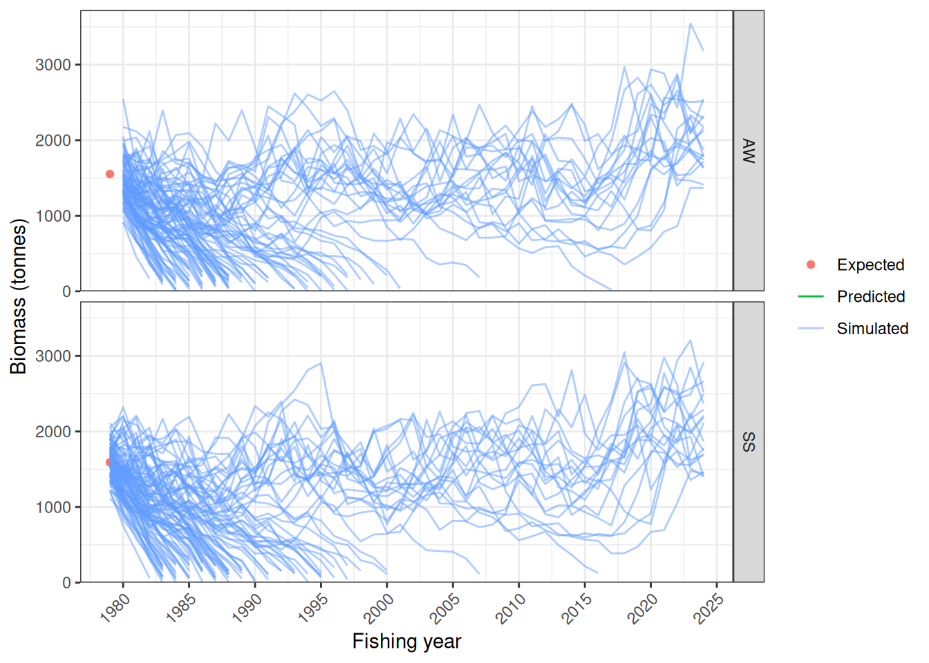
load(system.file("extdata", "base_biomass_AW.rda", package = "decamod"))
biomass_AW <- biomass_df %>% filter(Season == "AW")
biomass_AW$Base <- base_biomass_AW
ggplot(data = biomass_AW, aes(x = as.numeric(Year), y = Pred)) +
  geom_point(aes(y = Expected, color = "Expected")) +
  geom_line(aes(color = "Predicted")) +
  geom_line(aes(y = Base, color = "Base")) +
  scale_x_continuous(breaks = seq(1980, 2050, by = 5)) +
  scale_y_continuous(limits = c(0, NA), expand = expansion(mult = c(0, 0.05))) +
  theme(axis.text.x = element_text(angle = 45, vjust = 1, hjust = 1)) +
  labs(x = "Fishing year", y = "AW Biomass (tonnes)", color = NULL)
#> `geom_line()`: Each group consists of only one observation.
#> ℹ Do you need to adjust the group aesthetic?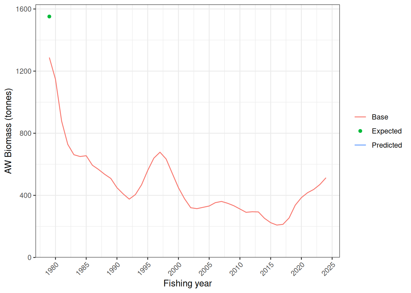
index_labels <- c("FSU", "FSU", "CELR", "CELR", "Logbook", "Logbook")

cpue_df <- data.frame(Period = data$cpue_time, Season = data$cpue_season,
                      Index = index_labels[data$cpue_q],
                      Obs = data$cpue_obs,
                      Pred = report$cpue_pred) %>%
  left_join(ys, by = join_by(Period, Season)) %>%
  mutate(Index = factor(Index, levels = c("FSU", "CELR", "Logbook"))) %>%
  mutate(Season = ifelse(Season == 1, "AW", "SS"))

set.seed(456)
sim_df <- NULL
for (i in 1:100) {
  df <- data.frame(Period = data$cpue_time, Season = data$cpue_season,
                   Index = index_labels[data$cpue_q],
                   Sim = obj$simulate(par = obj$env$last.par.best)$cpue_obs,
                   iter = i)
  sim_df <- bind_rows(sim_df, df)
}
sim_df <- sim_df %>%
  left_join(ys, by = join_by(Period, Season)) %>%
  mutate(Index = factor(Index, levels = c("FSU", "CELR", "Logbook"))) %>%
  mutate(Season = ifelse(Season == 1, "AW", "SS"))

ggplot(data = cpue_df, aes(x = as.numeric(Year), y = Obs)) +
  geom_point(aes(color = "Observed")) +
  geom_line(data = sim_df, aes(y = Sim, color = "Simulated", group = iter), alpha = 0.5) +
  geom_line(aes(y = Pred, group = interaction(Index, Season), color = "Predicted"), linewidth = 1.2) +
  facet_grid(Index ~ Season, scales = "free_y") +
  scale_x_continuous(breaks = seq(1980, 2050, by = 5)) +
  scale_y_continuous(limits = c(0, NA), expand = expansion(mult = c(0, 0.05))) +
  theme(axis.text.x = element_text(angle = 45, vjust = 1, hjust = 1)) +
  labs(x = "Fishing year", y = "CPUE", color = NULL)
#> `geom_line()`: Each group consists of only one observation.
#> ℹ Do you need to adjust the group aesthetic?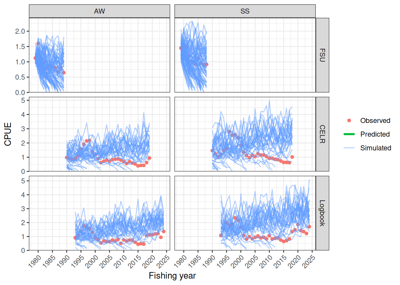
tibble(par = names(opt$par), value = exp(opt$par))
#> # A tibble: 11 × 2
#>    par              value
#>    <chr>            <dbl>
#>  1 log_r         0.261
#>  2 log_z         0.988
#>  3 log_K      2449.
#>  4 logit_D0      1.73
#>  5 log_q         0.000725
#>  6 log_q         0.000853
#>  7 log_q         0.000839
#>  8 log_q         0.00114
#>  9 log_q         0.000827
#> 10 log_q         0.00109
#> 11 log_sigmap    0.126
# obj$simulate(par = obj$env$last.par.best)$cpue_obs
# osa <- oneStepPredict(obj = obj, method = "oneStepGeneric", trace = FALSE)
# osa <- oneStepPredict(obj = obj, observation.name = "cpue_obs", method = "oneStepGeneric", trace = FALSE)
# qqnorm(osa$res); abline(0, 1)
# chk <- checkConsistency(obj = obj, hessian = TRUE, estimate = TRUE, n = 200)
# chk
# s <- summary(chk)
# s
# s$marginal$p.value
Bayesian inference
Using Cole Monnahan’s adnuts package, we can run the MCMC sampler. The adnuts package is a wrapper around the NUTS sampler in Stan. The objective function is evaluated using automatic differentiation (Kristensen et al. 2016).
# mcmc <- sample_sparse_tmb(
#   obj = obj, metric = "auto", iter = 4000, warmup = 3000, chains = 4, cores = 4,
#   control = list(adapt_delta = 0.99), init = "last.par.best", globals = decamod_globals())
# mcmc1 <- sample_snuts(
#   obj = obj, metric = "auto", num_samples = 1000, chains = 4, cores = 4,
#   control = list(adapt_delta = 0.99), init = "last.par.best",
#   # lower = Lwr, upper = Upr,
#   globals = list(get_growth_increment = get_growth_increment, drobust = drobust,
#                  jac_exp = jac_exp, jac_invlogit = jac_invlogit))
# library(priorsense)
# lp <- get_posterior(object = obj, posterior = mcmc1, pars = c("loglikes", "priors"), type = "array")
# samps <- extract_samples(fit = mcmc1, inc_lp = FALSE, as.list = FALSE)
# samps$lprior <- as.numeric(lp$priors[,,1])
# samps$log_lik <- as.numeric(lp$loglikes[,,1])
# psd <- create_priorsense_data(x = samps)
# powerscale_sensitivity(psd)
# powerscale_plot_dens(psd, variable = "log_galpha")
# powerscale_plot_ecdf(psd)
# powerscale_plot_quantities(psd)
#
# x <- example_powerscale_model()
# psd <- create_priorsense_data(x$draws)
# powerscale_sensitivity(psd)
# powerscale_plot_dens(psd)
# powerscale_plot_ecdf(psd)
# powerscale_plot_quantities(psd)
# plot_sampler_params(fit = mcmc1, plot = TRUE)
# pairs_rtmb(fit = mcmc1, order = "mismatch", pars = 1:5)
# pairs_rtmb(fit = mcmc1, order = "slow", pars = 1:5)
# plot_marginals(fit = mcmc1)
# plot_uncertainties(fit = mcmc1, log = TRUE, plot = TRUE)Likelihood profiles
The likelihood-profile helper needs to be expanded so the user can list what to report, as the current version does not work for the growth model.
# lincomb <- numeric(length(names(obj$par)))
# lc <- lincomb; lc[1] <- 1
# # prof_galpha1 <- tmbprofile2(obj = obj, lincomb = lc)
# prof_galpha1 <- TMB::tmbprofile(obj = obj, lincomb = lc)
# lc <- lincomb; lc[2] <- 1
# prof_galpha2 <- TMB::tmbprofile(obj = obj, lincomb = lc)
# plot(prof_galpha1)
# plot(prof_galpha2)
Hilborn, Ray, and Carl J. Walters. 1992. Quantitative Fisheries Stock Assessment: Choice, Dynamics and Uncertainty. Chapman; Hall. https://doi.org/10.1007/978-1-4615-3598-0.
Kristensen, Kasper, Anders Nielsen, Casper W. Berg, Hans Skaug, and Bradley M. Bell. 2016. “TMB: Automatic Differentiation and Laplace Approximation.” Journal of Statistical Software 70 (5): 1–21. https://doi.org/10.18637/jss.v070.i05.
Quinn, Terrance J., and Richard B. Deriso. 1999. Quantitative Fish Dynamics. Oxford University Press.
Schaefer, Milner B. 1954. “Some Aspects of the Dynamics of Populations Important to the Management of the Commercial Marine Fisheries.” Bulletin of the Inter-American Tropical Tuna Commission 1 (2): 27–56.