Bentley validation

Purpose

The original influ code developed by Nokome Bentley used the proto object system and GLMs (Bentley et al. 2012). That implementation is retained in influ2 as a frozen validation artefact, not as part of the package API. This vignette runs the old code explicitly and compares it with the model-neutral S3 engine.

The comparison uses the same simulated lobsters_per_pot example as the main vignette. Its deliberate shifts in sampled season, fishing depth, and soak time make the influence patterns more apparent. These are constructed teaching relationships, not empirical findings from a lobster fishery. A smaller frozen fixture remains in the test suite for fast regression testing.

Fit the common model

library(influ2)
data(lobsters_per_pot)

bentley_glm <- glm(
  lobsters ~ year + month + poly(depth, 3) + poly(soak, 3),
  family = poisson(link = "log"),
  data = lobsters_per_pot
)
new_diagnostic <- influ(bentley_glm, focus = "year")

The shared Poisson model provides a transparent test of agreement between implementations. The simulated catches have negative-binomial variation, so the Poisson uncertainty intervals are model-based and do not account for that overdispersion. Agreement of the calculations does not establish that their intervals have the intended coverage for these data.

The legacy source remains outside the namespace under inst/legacy. It is loaded into an isolated environment only for this comparison.

legacy_available <- requireNamespace("proto", quietly = TRUE)
if (legacy_available) {
  legacy_environment <- new.env(parent = globalenv())
  legacy_environment$proto <- proto::proto
  sys.source(
    system.file("legacy", "influ-proto.R", package = "influ2"),
    envir = legacy_environment
  )
  legacy_diagnostic <- legacy_environment$Influence$new(
    model = bentley_glm,
    data = lobsters_per_pot,
    response = "lobsters",
    focus = "year"
  )
  legacy_diagnostic$calc()
  # The original code predates R 4.0 and assumes that data.frame() converts
  # text to factors. Restore that historical plotting assumption here without
  # modifying the frozen implementation.
  legacy_diagnostic$influences$level <- factor(
    legacy_diagnostic$influences$level,
    levels = legacy_diagnostic$influences$level
  )
}
legacy_available
#> [1] TRUE

Influence plots

The left-hand figure is produced by the original proto method. The right-hand figure is produced from the new influ_diag. Both show monthly, depth, and soak-time influence as ratios centred on one across 18 years.

legacy_diagnostic$influPlot()

plot(
  new_diagnostic,
  type = "influence",
  term = c("month", "poly(depth, 3)", "poly(soak, 3)"),
  scale = "ratio"
) +
  facet_grid(term ~ scale)

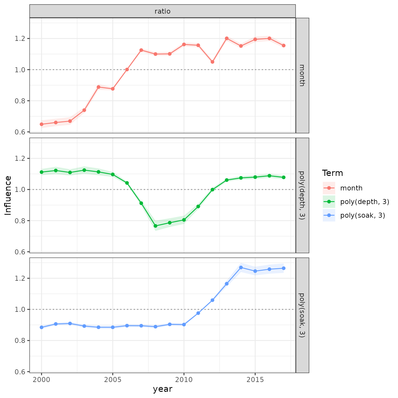
Influence plots for the lobster example from the original Bentley proto implementation (left) and the new influ2 engine (right).

CDI plots

The complete coefficient-distribution-influence display combines the fitted effect, the distribution of observations, and the resulting influence. Both figures below use month as the model term and year as the focus.

Both top-left panels now show the same relative monthly effects: log-scale term contributions are centred on the observed monthly distribution, then exponentiated. The reference is one on a logarithmic axis. This removes the arbitrary choice of month 1 as the zero coefficient; a relative effect of 1.2 means a 20% higher monthly contribution to expected catch than the reference. The legacy label “Coefficient” and the new label “Relative month effect” describe the same fitted quantity in this example.

The interval widths deliberately differ. The original plot uses plus or minus one standard error on the centred log scale, followed by exponentiation. The new plot uses approximate 95% confidence intervals, including uncertainty in the estimated centre and its covariance with each month’s effect. Its annual influence panel also includes uncertainty intervals.

legacy_diagnostic$cdiPlot(term = "month")
plot(new_diagnostic, type = "cdi", term = "month")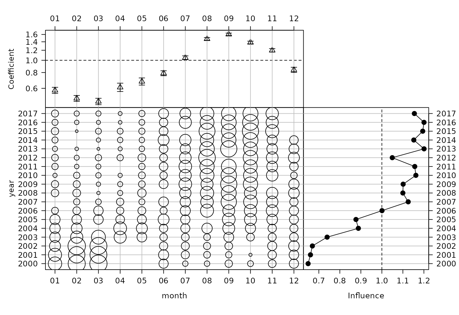

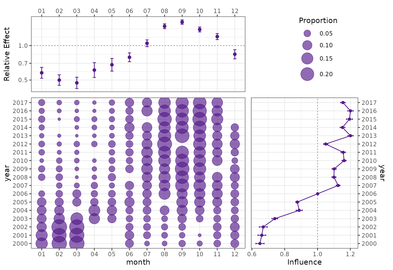
CDI plots for month from Bentley proto (left) and influ2 (right). The centred relative-effect points agree; legacy top-panel bars use plus or minus one standard error, while influ2 uses 95% confidence intervals.

To inspect the earlier reference-coded display instead, use coefficient_reference = "model". In this GLM that puts month 1 at zero and shows the other months relative to it, on the log scale. Alternatively, coefficient_scale = "link" keeps the new centring but displays additive log effects. Neither option changes the annual influence calculations.

Numerical agreement

First, compare the top-panel centred log effects and their standard errors. Exponentiating the estimates gives the matching relative-effect points shown above. Checking the standard errors separately verifies that the difference between the plotted intervals comes from their stated coverage.

legacy_coefficients <- aggregate(
  legacy_diagnostic$preds[c("fit.month", "se.fit.month")],
  list(level = legacy_diagnostic$preds$month),
  mean
)
names(legacy_coefficients) <- c(
  "level", "centred_estimate_legacy", "centred_std_error_legacy"
)
current_coefficients <- subset(
  new_diagnostic$coefficients,
  term == "month",
  select = c(level, centred_estimate, centred_std_error)
)
coefficient_comparison <- merge(
  legacy_coefficients, current_coefficients, by = "level"
)
coefficient_comparison$relative_effect <- exp(
  coefficient_comparison$centred_estimate
)
coefficient_comparison
#>    level centred_estimate_legacy centred_std_error_legacy centred_estimate
#> 1     01             -0.54808969               0.05585420      -0.54808969
#> 2     02             -0.69438688               0.05387027      -0.69438688
#> 3     03             -0.75016486               0.05788165      -0.75016486
#> 4     04             -0.49270009               0.07588558      -0.49270009
#> 5     05             -0.38650045               0.06486564      -0.38650045
#> 6     06             -0.23598670               0.04500541      -0.23598670
#> 7     07              0.04580356               0.03468835       0.04580356
#> 8     08              0.38848291               0.02469844       0.38848291
#> 9     09              0.47247605               0.02238562       0.47247605
#> 10    10              0.32365699               0.02475293       0.32365699
#> 11    11              0.18089320               0.03091266       0.18089320
#> 12    12             -0.17448551               0.04703920      -0.17448551
#>    centred_std_error relative_effect
#> 1         0.05585420       0.5780530
#> 2         0.05387027       0.4993805
#> 3         0.05788165       0.4722887
#> 4         0.07588558       0.6109745
#> 5         0.06486564       0.6794304
#> 6         0.04500541       0.7897912
#> 7         0.03468835       1.0468687
#> 8         0.02469844       1.4747418
#> 9         0.02238562       1.6039608
#> 10        0.02475293       1.3821731
#> 11        0.03091266       1.1982872
#> 12        0.04703920       0.8398890
stopifnot(
  max(abs(coefficient_comparison$centred_estimate_legacy -
    coefficient_comparison$centred_estimate)) < 1e-8,
  max(abs(coefficient_comparison$centred_std_error_legacy -
    coefficient_comparison$centred_std_error)) < 1e-8
)

The old and new engines are also compared directly on all 54 year-by-term contrasts in the lobster example. Routine testthat tests retain both this realistic comparison and a smaller frozen numerical fixture.

legacy <- reshape(
  as.data.frame(legacy_diagnostic$influences),
  direction = "long",
  varying = names(legacy_diagnostic$influences)[-1],
  v.names = "link_influence_legacy",
  timevar = "term",
  times = names(legacy_diagnostic$influences)[-1]
)
rownames(legacy) <- NULL

current <- subset(
  influ_effects(new_diagnostic),
  term != "year" & scale == "link",
  select = c(level, term, estimate)
)
names(current)[names(current) == "estimate"] <- "link_influence_new"

comparison <- merge(
  legacy[c("level", "term", "link_influence_legacy")],
  current,
  by = c("level", "term")
)
comparison$natural_influence_legacy <- exp(comparison$link_influence_legacy)
comparison$absolute_difference <- abs(
  comparison$link_influence_legacy - comparison$link_influence_new
)
head(comparison)
#>   level           term link_influence_legacy link_influence_new
#> 1  2000          month           -0.43233253        -0.43233253
#> 2  2000 poly(depth, 3)            0.10599428         0.10599428
#> 3  2000  poly(soak, 3)           -0.12260121        -0.12260121
#> 4  2001          month           -0.41522396        -0.41522396
#> 5  2001 poly(depth, 3)            0.11516257         0.11516257
#> 6  2001  poly(soak, 3)           -0.09831081        -0.09831081
#>   natural_influence_legacy absolute_difference
#> 1                0.6489935        5.551115e-17
#> 2                1.1118155        1.387779e-17
#> 3                0.8846164        0.000000e+00
#> 4                0.6601924        0.000000e+00
#> 5                1.1220558        1.387779e-17
#> 6                0.9063672        0.000000e+00
max(comparison$absolute_difference)
#> [1] 1.110223e-16
stopifnot(max(comparison$absolute_difference) < 1e-8)

The same validation covers the two scalar metrics from the original implementation. overall summarises mean absolute influence, while trend summarises the ordered change through the focus levels.

legacy_metrics <- subset(
  legacy_diagnostic$summary,
  term != "intercept" & term != "year",
  select = c(term, overall, trend)
)
new_metrics <- reshape(
  influ_metrics(new_diagnostic)[c("term", "metric", "estimate")],
  direction = "wide",
  idvar = "term",
  timevar = "metric"
)
names(new_metrics) <- sub("^estimate\\.", "", names(new_metrics))
metric_comparison <- merge(
  legacy_metrics,
  new_metrics,
  by = "term",
  suffixes = c("_legacy", "_new")
)
metric_comparison
#>             term overall_legacy trend_legacy overall_new    trend_new
#> 1          month      0.2001537  0.037814471   0.2001537  0.037814471
#> 2 poly(depth, 3)      0.1164328 -0.004176475   0.1164328 -0.004176475
#> 3  poly(soak, 3)      0.1409172  0.024185229   0.1409172  0.024185229
stopifnot(
  max(abs(metric_comparison$overall_legacy - metric_comparison$overall_new)) < 1e-8,
  max(abs(metric_comparison$trend_legacy - metric_comparison$trend_new)) < 1e-8
)

The final overlay makes exact agreement visually apparent: legacy results are points, and new results are lines.

ggplot(comparison, aes(x = level, group = term)) +
  geom_hline(yintercept = 1, linetype = 3, colour = "grey55") +
  geom_point(
    aes(y = natural_influence_legacy, shape = "Legacy proto"),
    size = 3
  ) +
  geom_line(
    aes(y = exp(link_influence_new), colour = "New influ2"),
    linewidth = 0.9
  ) +
  facet_wrap(~term, ncol = 1, scales = "free_y") +
  scale_colour_manual(values = c("New influ2" = "#0072B2")) +
  scale_shape_manual(values = c("Legacy proto" = 21)) +
  labs(
    x = "Year",
    y = "Influence ratio",
    colour = NULL,
    shape = NULL
  ) +
  theme(legend.position = "bottom")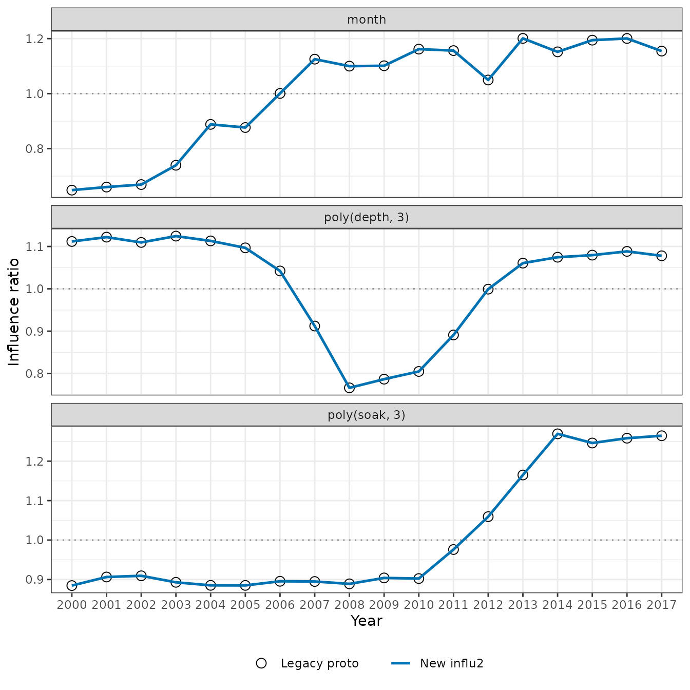

Direct overlay of legacy Bentley influence values and new influ2 results for the lobster example.

References

Bentley, Nokome, Terese H. Kendrick, Paul J. Starr, and Paul A. Breen. 2012. “Influence Plots and Metrics: Tools for Better Understanding Fisheries Catch-Per-Unit-Effort Standardizations.” ICES Journal of Marine Science 69 (1): 84–88. https://doi.org/10.1093/icesjms/fsr174.