CPUE indices

An assessment-ready table

cpue_index() calculates the expected response for a fixed reference population in every year. It produces the familiar assessment columns: Year, Mean, Median, SD, CV, Qlower, and Qupper, alongside method, distribution, and link metadata. The result is an influ_index object; index_table() gives a reporting table, omitting an unavailable median by default. as.data.frame() retains the full, stable schema for existing code.

For two regional series from one fitted model, see Regional CPUE indices. That worked example groups four statistical areas into two regions, holds reference weights fixed, and checks the annual uncertainty against native predictions.

This is a different quantity from the centred year-effect contrasts in the influence and step plots. Both are useful, but neither is automatically an area-integrated abundance or biomass index.

Both cpue_index() and the separate integrate_index() work with GLM, GAM, glmmTMB, complete brms, sdmTMB, and univariate tinyVAST fits. Spatial effects are not required for either calculation. The difference is the question: standardisation produces a weighted mean, whereas integration produces an area-weighted total over a stated domain.

We use the same simulated lobster catches as the main article. The model below includes a monthly random intercept and a negative-binomial observation distribution. No simulation of new catches is needed for its index.

data(lobsters_per_pot)
lobster_model <- glmmTMB::glmmTMB(
  lobsters ~ year + poly(depth, 3) + poly(soak, 3) + (1 | month),
  family = glmmTMB::nbinom2(), data = lobsters_per_pot
)

We explicitly choose median observed depth and a 24-hour soak. The year column is omitted: cpue_index() repeats this same profile in every observed year. The monthly random effect is set to zero. That represents a zero-effect month on the link scale, not the average response across the population of months. These choices belong to the scientific definition of the index.

reference <- data.frame(depth = median(lobsters_per_pot$depth), soak = 24)
lobster_index <- cpue_index(
  lobster_model, year = "year", method = "standardised",
  reference_data = reference, units = "lobsters per pot"
)
knitr::kable(index_table(lobster_index), digits = 3)

Year	Mean	SD	CV	Qlower	Qupper	Method	Distribution	Link
2000	1.674	0.238	0.142	1.267	2.212	standardised	nbinom2	log
2001	1.744	0.247	0.142	1.321	2.303	standardised	nbinom2	log
2002	1.815	0.254	0.140	1.380	2.387	standardised	nbinom2	log
2003	1.387	0.189	0.136	1.062	1.812	standardised	nbinom2	log
2004	1.572	0.214	0.136	1.204	2.053	standardised	nbinom2	log
2005	1.310	0.185	0.141	0.993	1.729	standardised	nbinom2	log
2006	1.167	0.158	0.136	0.895	1.522	standardised	nbinom2	log
2007	1.184	0.161	0.136	0.907	1.545	standardised	nbinom2	log
2008	1.172	0.164	0.140	0.891	1.541	standardised	nbinom2	log
2009	1.123	0.157	0.140	0.853	1.477	standardised	nbinom2	log
2010	1.219	0.167	0.137	0.932	1.595	standardised	nbinom2	log
2011	1.379	0.189	0.137	1.055	1.803	standardised	nbinom2	log
2012	1.214	0.170	0.140	0.922	1.598	standardised	nbinom2	log
2013	1.372	0.187	0.136	1.051	1.792	standardised	nbinom2	log
2014	1.259	0.171	0.136	0.965	1.642	standardised	nbinom2	log
2015	1.067	0.146	0.137	0.816	1.395	standardised	nbinom2	log
2016	1.094	0.148	0.135	0.840	1.426	standardised	nbinom2	log
2017	1.118	0.153	0.137	0.855	1.462	standardised	nbinom2	log

method = "standardized" works identically. There is no need to refit a model when printing, exporting, or plotting this result.

plot_index(lobster_index)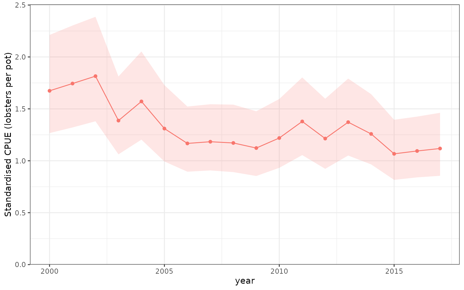

Standardised expected lobsters per pot at the stated depth and soak-time reference profile, with the monthly random effect set to zero. The ribbon is a pointwise 95% delta-method confidence interval for the index, not the spread of individual catches.

What do the uncertainty columns mean?

For GLMs, GAMs, and glmmTMB, Mean is the fitted expected-response estimate; SD is its propagated standard error. CV is SD / Mean when the estimate is positive. Median is deliberately missing: an MLE is not a posterior median. Positive estimates use log-scale delta-method intervals.

For a complete brms fit, Mean, Median, SD, and the interval columns summarise posterior draws of the expected-response index. They do not describe the mean and median of individual catches. The native posterior_epred() calculation combines the distributional parameters, including zero and positive components where appropriate, within each draw.

# Use an existing complete fit, not the compact influence-vignette fixture.
bayesian_index <- cpue_index(
  complete_brms_fit, year = "year", reference_data = reference,
  ndraws = 1000, batch_size = 250, draw_batch_size = 100,
  retain = "summary"
)
as.data.frame(bayesian_index)

Prediction batches preserve the same draw identities across years and reference rows. Only the annual summaries and their two small covariance matrices are retained by default. Setting retain = "draws" retains a draw-by-year matrix, not the much larger reference-row-by-draw prediction matrix. The fitted model and reference data are not embedded in the output object. Native prediction routines can still allocate their own working memory.

uncertainty = "none" omits uncertainty summaries. For frequentist models this also avoids covariance propagation. For brms it still averages existing posterior expected-response draws, so it is not a shortcut that substitutes posterior-mean coefficients and changes the quantity being estimated.

Lognormal assessment parameters

Some assessments accept an index median and a log-scale SD, whereas others accept an arithmetic mean and CV. index_table(index, format = "lognormal") provides an explicit marginal lognormal approximation from the index’s Mean and SD:

$$s^2 = \log(1 + (\mathrm{SD}/\mathrm{Mean})^2),\qquad m = \log(\mathrm{Mean}) - s^2/2.$$

The additional columns are Meanlog = m, SDlog = s, and LognormalMedian = exp(m). Substituting them into the usual lognormal moment formulae recovers the input mean and variance. They describe uncertainty in the annual index, not the distribution or residual dispersion of the fitted response. A negative-binomial CPUE model can therefore supply a lognormal assessment approximation without becoming a lognormal response model.

assessment_marginals <- index_table(lobster_index, format = "lognormal")
knitr::kable(assessment_marginals[c("Year", "Mean", "SD", "CV",
  "Meanlog", "SDlog", "LognormalMedian")], digits = 3)

Year	Mean	SD	CV	Meanlog	SDlog	LognormalMedian
2000	1.674	0.238	0.142	0.505	0.142	1.657
2001	1.744	0.247	0.142	0.546	0.141	1.727
2002	1.815	0.254	0.140	0.586	0.139	1.798
2003	1.387	0.189	0.136	0.318	0.136	1.374
2004	1.572	0.214	0.136	0.443	0.136	1.557
2005	1.310	0.185	0.141	0.260	0.141	1.297
2006	1.167	0.158	0.136	0.146	0.135	1.157
2007	1.184	0.161	0.136	0.159	0.135	1.173
2008	1.172	0.164	0.140	0.149	0.139	1.160
2009	1.123	0.157	0.140	0.106	0.139	1.112
2010	1.219	0.167	0.137	0.189	0.136	1.208
2011	1.379	0.189	0.137	0.312	0.136	1.366
2012	1.214	0.170	0.140	0.184	0.139	1.202
2013	1.372	0.187	0.136	0.307	0.136	1.359
2014	1.259	0.171	0.136	0.221	0.135	1.247
2015	1.067	0.146	0.137	0.056	0.136	1.057
2016	1.094	0.148	0.135	0.081	0.134	1.084
2017	1.118	0.153	0.137	0.103	0.136	1.108

stopifnot(isTRUE(all.equal(
  exp(assessment_marginals$Meanlog + assessment_marginals$SDlog^2 / 2),
  assessment_marginals$Mean
)))

An actual posterior Median, where available, is preserved separately; it is not overwritten by LognormalMedian. Frequentist reporting omits the missing Median by default, while include_median = "always" retains that column. This resolves the empty-column presentation without inventing posterior summaries. Non-positive means, invalid SDs, preview results, and year-effect contrasts cannot produce this lognormal table.

The moment-matched Meanlog is not log(Mean). Similarly, SDlog is not generally the log-index SE from the joint calculation below. Choose the assessment likelihood’s convention explicitly: do not silently substitute one centre or uncertainty measure for the other.

Joint annual uncertainty

index_vcov(index) (or vcov(index)) returns covariance among log annual indices; scale = "response" gives covariance in the reported units. The calculation uses the same reference population, random-effect target, and normalisation as the table. It never refits the model or simulates new observations. The diagonal of the response matrix matches SD^2.

Backend	Joint covariance calculation
GLM, GAM, glmmTMB	Delta method through the weighted annual response means; log-index gradients for log covariance.
brms	Sample covariance of annual posterior expected-response draws; take logs of those same draws for log covariance.
sdmTMB, tinyVAST	Sample covariance of joint Gaussian parameter/field simulations of the annual index; these are not MCMC draws.

Shared parameters and fields can correlate estimates in different years. This is not a residual autocorrelation estimate. A matrix cannot be recovered from marginal SDs alone; old saved summaries without covariance must be recalculated from their fitted models. uncertainty = "none" deliberately does not provide a matrix. Log covariance requires positive estimates and, for simulation methods, positive draws; values are not clipped to pass this check. A response-scale matrix can still exist when log covariance cannot.

Sigma <- index_vcov(lobster_index, require_pd = TRUE)
stopifnot(identical(rownames(Sigma), as.character(lobster_index$table$Year)))
stopifnot(isTRUE(all.equal(
  unname(diag(index_vcov(lobster_index, scale = "response"))),
  lobster_index$table$SD^2
)))

# Select and order both dimensions together, then match the table to them.
selected_years <- tail(lobster_index$table$Year, 5)
selected_Sigma <- index_vcov(lobster_index, years = selected_years)
selected_table <- index_table(lobster_index)[
  match(rownames(selected_Sigma), lobster_index$table$Year), ]
stopifnot(identical(selected_table$Year, rownames(selected_Sigma)))

plot(lobster_index, type = "correlation")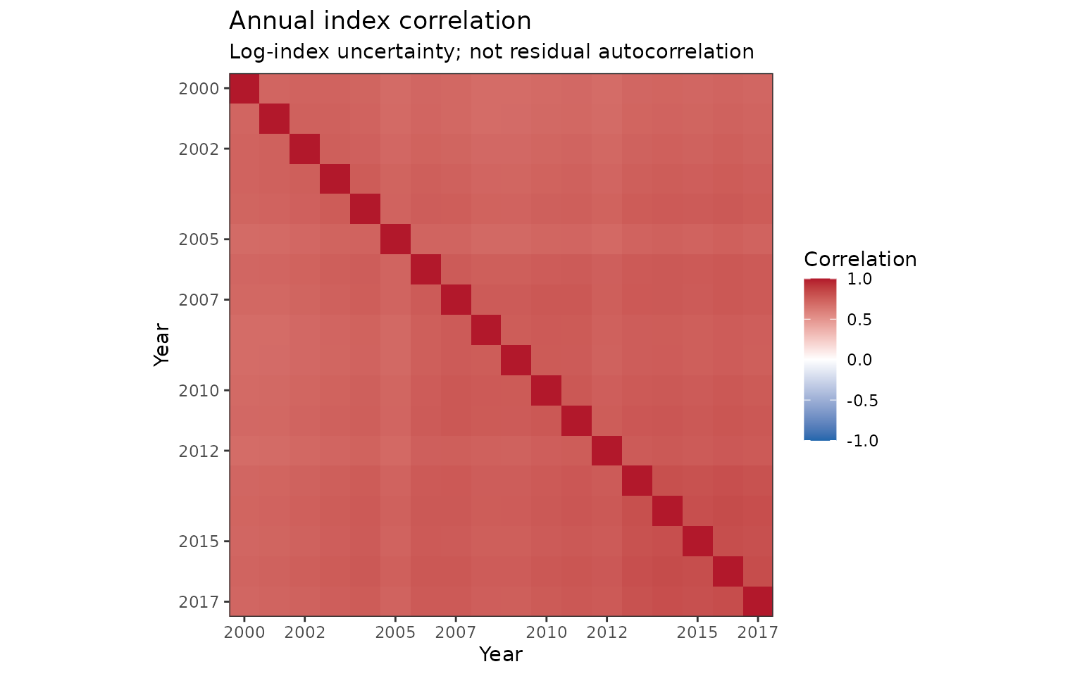

Correlation among the unscaled annual log CPUE indices. The off-diagonal cells preserve dependence from the shared fitted model; these are not correlations among observed responses or residuals. The full covariance, rather than this unitless display, is the assessment input.

For a covariance display, use plot(lobster_index, type = "covariance"). The main article shows both and an example assessment-input bundle. Keeping estimated dependence is preferable to discarding it when the joint uncertainty model is appropriate, but it is not a guarantee of improved stock-status estimates. Hoyle et al. (2024) discuss covariance propagation in index construction (Section 5.8) and the additional sources of uncertainty an assessment may need (Section 5.5).

Retain rescale = "raw" for an assessment with an estimated catchability. Draw-wise geometric-mean normalisation removes a common level and makes the log covariance singular. The default extractor permits positive semidefinite matrices for inspection; require_pd = TRUE rejects a matrix that cannot safely be Cholesky-factorised. It never repairs eigenvalues or adds diagonal jitter. Too few draws or other model constraints can also produce rank deficiency.

Area integration retains the same matrices. Multiplying by a known positive area or unit-conversion constant multiplies response covariance by its square and leaves log covariance unchanged. Reference-weight and catchability uncertainty, additional assessment process/error variance, and cross-series covariance between independently calculated objects are not supplied. For brms, the matrix summarises a posterior, not a prior-free likelihood; check prior reuse before treating it as new independent assessment evidence.

A common reference population and relative scaling

Supply multiple reference rows and explicit weights to standardise over a population. Predictions are averaged on the response scale, after applying the inverse link, using the same weights in each year. The function never chooses missing factor values or an exposure variable on the user’s behalf.

population <- data.frame(depth = c(25, 45, 65), soak = 24)
relative_index <- cpue_index(
  lobster_model, year = "year", reference_data = population,
  reference_weights = c(0.2, 0.5, 0.3), rescale = 1
)
geo_mean(relative_index$table$Mean)
#> [1] 1

The weights here are illustrative population proportions, not cell areas. For models of catch with an exposure offset, put the offset in the formula and explicitly supply the desired exposure in the reference data. For a per-pot index from a catch model, this would usually be one pot. This example already models catches from individual pots.

rescale = 1 normalises across all returned years. Frequentist uncertainty includes covariance with that denominator. For brms, each complete annual draw is normalised before summarising; the geometric mean of the resulting posterior-mean column need not be exactly one. Do not separately normalise the mean, median, and interval columns: that changes their relative scales.

geo_mean() is also available independently. It calculates on the log scale to avoid numerical overflow, includes zeros, and supports na.rm = TRUE. Negative values and infinities are rejected.

Comparing models

plot_compare() accepts calculated influ_index objects. Use the same response definition, reference population, weights, exposure, and scale. Automatic metadata checks cannot establish scientific comparability.

linear_model <- glmmTMB::glmmTMB(
  lobsters ~ year + depth + soak + (1 | month),
  family = glmmTMB::nbinom2(), data = lobsters_per_pot
)
linear_index <- cpue_index(linear_model, reference_data = reference,
  units = "lobsters per pot")
plot_compare(list(Curved = lobster_index, Linear = linear_index))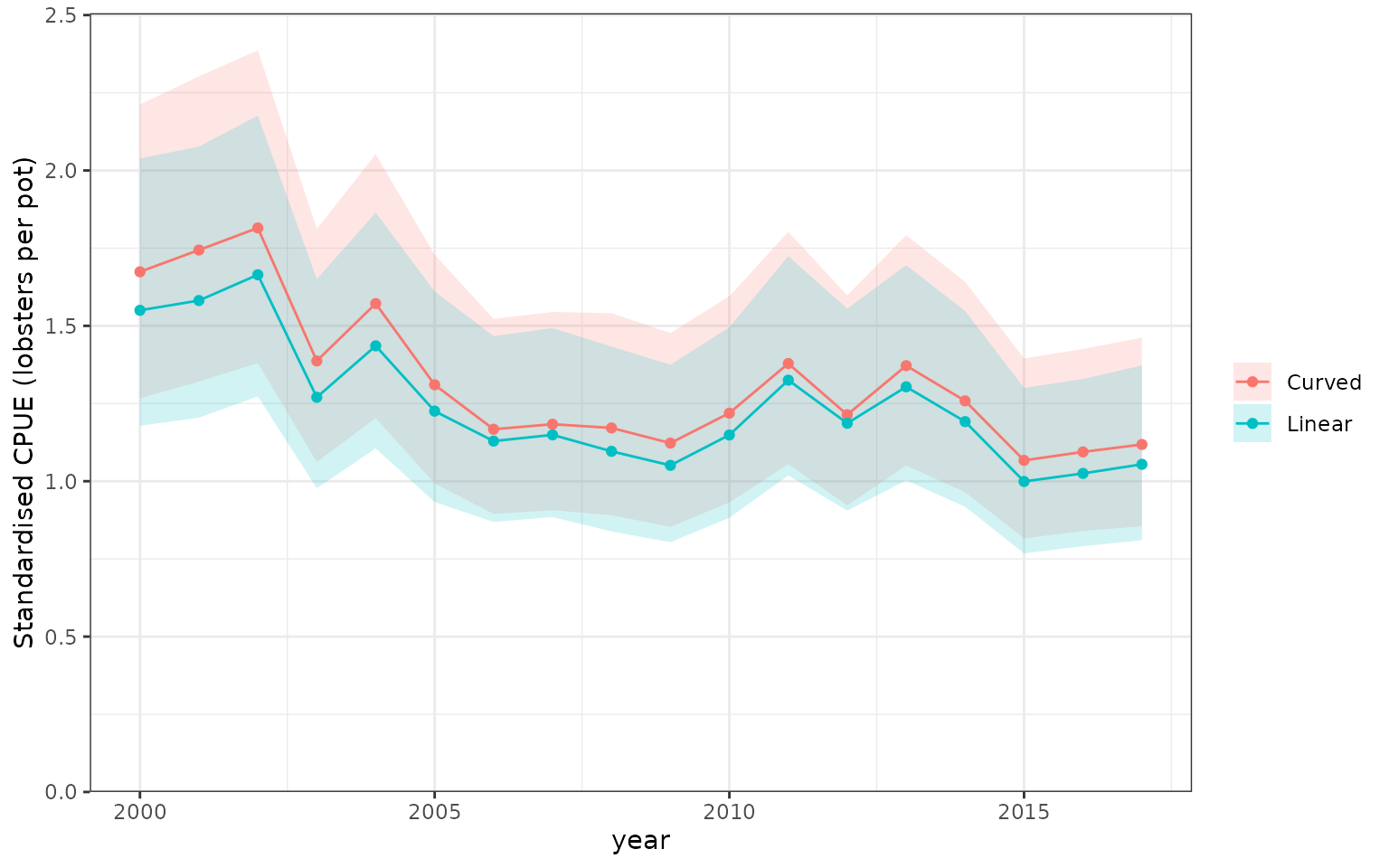

Expected-response indices from two negative-binomial glmmTMB candidates at the same reference profile. Both use the same monthly random-effect convention and response units. Intervals describe each index separately, not uncertainty in the difference between the models.

When supplied fitted models or influ_diag objects instead, plot_compare() keeps its existing year-effect-contrast behaviour. It does not silently switch to response predictions. plot_step() also remains a year-effect comparison.

Current boundaries

Response standardisation and area integration support all six backends above, subject to model-structure checks. glmmTMB indices require a converged ML fit and do not yet support random effects in the zero component. brms autocorrelation and Gaussian-process predictions need a separate joint-prediction adapter. GAM smooths are evaluated as fitted, including random-effect smooths; their target can differ from the zero-group-effect convention used for glmmTMB and brms.

For binomial GLMs and glmmTMB, native response predictions are probabilities. For brms binomial models they are expected counts at the reference number of trials: supply one trial for a per-trial comparison. Quasi families and transformed responses are not supported here. Use an explicit lognormal family instead of asking the package to guess a back-transformation.

For sdmTMB and tinyVAST, response predictions include fitted spatial and spatiotemporal fields by default. spatial_fields can select "all", "spatial", "spatiotemporal", or "none" without refitting. Joint Gaussian parameter/field draws preserve dependence across cells and years. These are not MCMC draws. The reported frequentist Mean is a plug-in expectation, with simulation-based uncertainty, not a Laplace bias-corrected total. Native sdmTMB::get_index() and tinyVAST::integrate_output() offer bias correction; agreement checks use their uncorrected estimates to compare the same calculation. Frequentist Median remains undefined in the full schema and is omitted from the default reporting table.

All calculations use a fixed common reference domain in the observed years. They do not forecast or automatically supply year-varying environmental covariates. Multivariate tinyVAST response integration and sdmTMB nonlocal covariate operators are rejected explicitly. Integration over a new population of latent random effects is a different target, not implied by these methods.

Area integration for ordinary and spatial models

No specialist spatiotemporal model is required. Given a prediction grid, integrate_index() sums cell area * expected response in each year. The same routine works for a GLM with no spatial effects, a GAM with a spatial smooth, or any of the other supported model classes. A model without a spatial term cannot reveal spatial variation that is not explained by its other predictors, but its predictions can still be integrated.

This separate simulated example has a density response in kg/km², so multiplying by cell areas in km² yields kg. It is not a conversion of the lobster pot catches above into biomass. The changing survey footprint is deliberately imbalanced.

set.seed(710)
survey <- data.frame(year = factor(rep(2011:2016, each = 100)))
survey$x <- runif(nrow(survey), 0, 10)
survey$y <- runif(nrow(survey), 0, 10)
survey$depth <- 20 + 3 * survey$x + 2 * survey$y
eta <- 2 + 0.08 * as.integer(survey$year) - 0.012 * survey$depth +
  0.7 * sin(survey$x / 2) * cos(survey$y / 3)
survey$density <- rgamma(nrow(survey), shape = 5, scale = exp(eta) / 5)
sampling_centre <- 1 + 8 * (as.integer(survey$year) - 1) / 5
survey <- survey[runif(nrow(survey)) <
  0.35 + 0.65 * exp(-(survey$x - sampling_centre)^2 / 8), ]

# One row per 0.5 x 0.5 km cell: 400 cells over a 100 km² domain.
density_grid <- expand.grid(x = seq(0.25, 9.75, by = 0.5),
                           y = seq(0.25, 9.75, by = 0.5))
density_grid$depth <- 20 + 3 * density_grid$x + 2 * density_grid$y
density_grid$area_km2 <- 0.25

gam_density <- mgcv::gam(density ~ year + s(x, y, k = 20),
  family = Gamma(link = "log"), data = survey, method = "REML")
glm_density <- glm(density ~ year + depth,
  family = Gamma(link = "log"), data = survey)

gam_total <- integrate_index(gam_density, density_grid, area = "area_km2",
  area_units = "km^2", response_units = "kg/km^2", units = "kg")
glm_total <- integrate_index(glm_density, density_grid, area = "area_km2",
  area_units = "km^2", response_units = "kg/km^2", units = "kg")
knitr::kable(index_table(gam_total), digits = 3)

Year	Mean	SD	CV	Qlower	Qupper	Method	Distribution	Link
2011	472.599	29.482	0.062	418.208	534.065	integrated	Gamma	log
2012	548.591	30.319	0.055	492.273	611.352	integrated	Gamma	log
2013	561.066	30.956	0.055	503.559	625.141	integrated	Gamma	log
2014	631.213	34.297	0.054	567.446	702.144	integrated	Gamma	log
2015	635.394	38.429	0.060	564.368	715.359	integrated	Gamma	log
2016	758.069	43.860	0.058	676.800	849.096	integrated	Gamma	log

plot_compare(list(`Spatial GAM` = gam_total, `Depth GLM` = glm_total))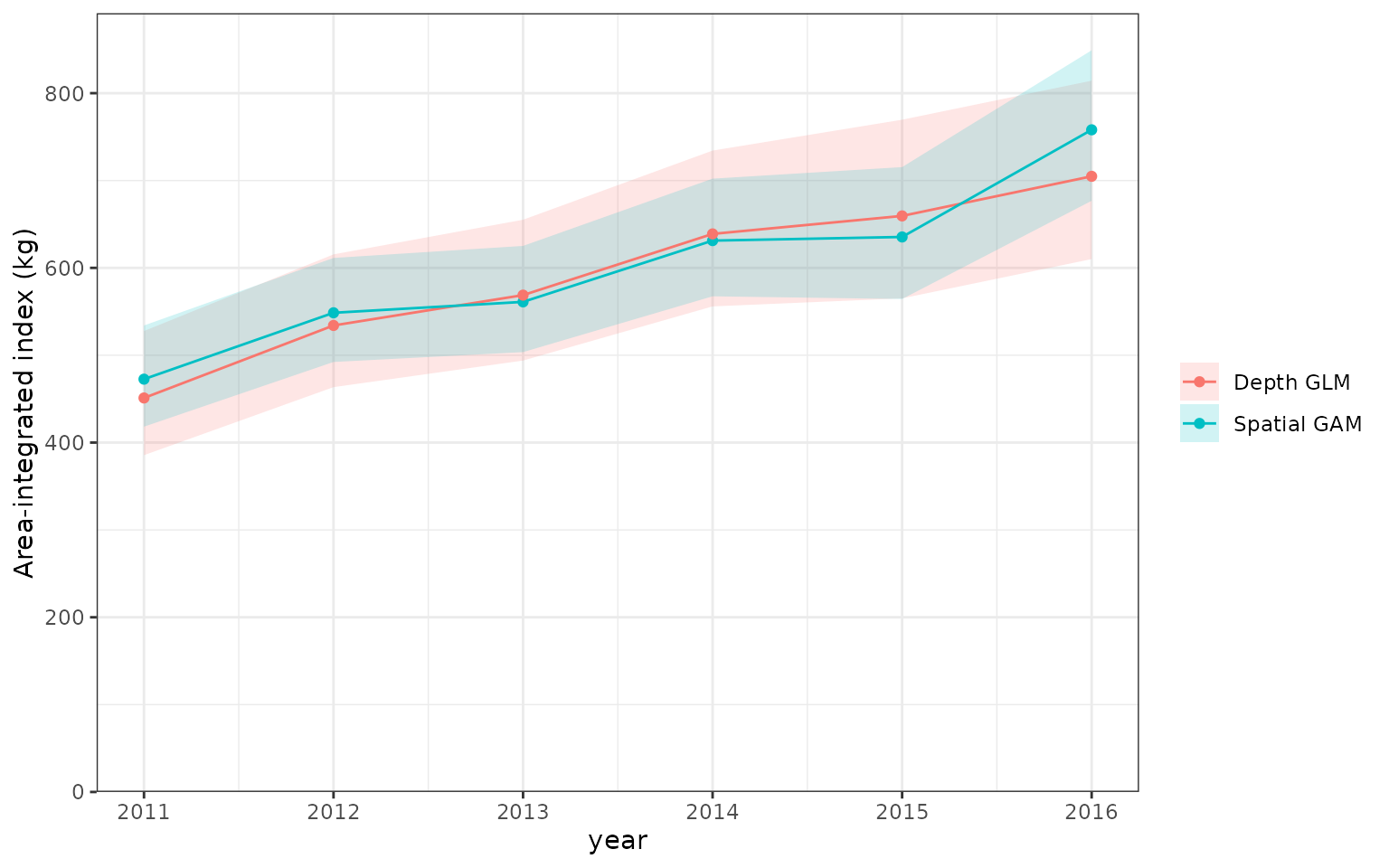

Area-integrated expected density over the same 100 km² domain, comparing a GAM with a spatial smooth against a GLM with a depth effect but no explicit spatial term. Both return totals in kg under the simulated density units. Pointwise 95% confidence intervals propagate joint coefficient uncertainty; they do not describe new catches or uncertainty in the difference between models.

Replace the fitted model with a glmmTMB or complete brms fit to use exactly the same integration call. The spatial article executes both index calculations for sdmTMB and tinyVAST, including their fields.

Area integration and area-weighted standardisation are related, but not identical: with no catchability conversion, the total is the area-weighted mean times total area. Their units differ. rescale = 1 gives a relative series and includes the shared normalising denominator in uncertainty calculations.

Exposure, catchability, and repeated seasons

Integrating kg/tow over km² gives an area-weighted CPUE index, not kg of fish. Either model a density already expressed per km² or supply a defensible known catchability conversion with compatible units. The package divides predictions by that conversion; it does not estimate catchability or its uncertainty. It also does not infer cell areas from longitude and latitude: use suitable geodesic or equal-area calculations outside this function.

If each cell appears in several seasonal reference rows, provide averaging_weights that sum to one within each cell. For example, four equally weighted quarters need averaging_weights = 1 / 4. Without this adjustment, repeating the full cell area four times computes a sum over four seasons rather than an annual mean surface. This is also relevant to month-by-area GAM grids: the integration weights must represent the intended seasonal and spatial target.

seasonal_total <- integrate_index(seasonal_model, quarter_grid,
  area = "area_km2", averaging_weights = 1 / 4,
  area_units = "km^2", response_units = "kg/km^2", units = "kg")

Only the compact annual table and covariance matrices are retained by default. Spatial and brms indices can retain annual draws with retain = "draws"; grid-by-draw arrays are not stored. Independent cell standard errors are never added together. All area, covariate, and seasonal weights are treated as known, and valid units, domain coverage, and extrapolation remain scientific decisions for the analyst.

References

Hoyle, Simon D., Robert A. Campbell, Nicholas D. Ducharme-Barth, et al. 2024. “Catch Per Unit Effort Modelling for Stock Assessment: A Summary of Good Practices.” Fisheries Research 269: 106860. https://doi.org/10.1016/j.fishres.2023.106860.