Hurdle and zero-inflated models • influ2

Why retain components?

A hurdle or delta model has an occurrence component and a positive component. Its unconditional expected response is

$E(Y) = \Pr(Y > 0) E(Y \mid Y > 0).$

A zero-inflated count model instead combines an additional-zero probability with a count distribution:

$E(Y) = \{1 - \Pr(\text{extra zero})\}\mu_{\text{count}}.$

An influence diagnostic should show both component-specific effects and the combined change in expected response. Treating one component as though it were the complete CPUE index can obscure why an index changed.

brms hurdle-lognormal example

A hurdle-lognormal model can be fitted with separate formulae for positive catch and the probability of a zero:

set.seed(42)
n <- 1000
year_effect <- data.frame(
  year = 1995:2015,
  value = rnorm(21)
)
sampled_year <- year_effect[
  sample(seq_len(nrow(year_effect)), size = n, replace = TRUE),
]
group <- sample(c("treat", "placebo"), size = n, replace = TRUE)
simulated_cpue <- data.frame(
  y = (1 - rbinom(n, 1, 0.3)) * rlnorm(
    n,
    meanlog = 2 + ifelse(group == "treat", 0.9, 0) + sampled_year$value,
    sdlog = 0.2
  ),
  year = factor(sampled_year$year),
  group = group
)

fit <- brms::brm(
  brms::bf(y ~ year + group, hu ~ 1),
  data = simulated_cpue,
  family = brms::hurdle_lognormal(),
  chains = 4,
  cores = 2,
  iter = 2000,
  warmup = 1000,
  seed = 42,
  control = list(adapt_delta = 0.99, max_treedepth = 12),
  file = "m1",
  file_refit = "on_change"
)

The vignette uses the pre-fitted object supplied with its source. Joint posterior draws are reduced directly to compact component and unconditional-mean contrasts.

library(influ2)
fit <- readRDS(system.file(
  "extdata", "brms-fixtures", "m1.rds", package = "influ2"
))
hurdle_diagnostic <- influ(fit, focus = "year", ndraws = 250)
unique(hurdle_diagnostic$influence$component)
#> [1] "positive"           "unconditional_mean"
summary(hurdle_diagnostic)
#> Influence diagnostic summary
#>   Backend: brms
#>   Family:  hurdle lognormal (identity)
#>   Focus:   year
#> 
#>   term                    component maximum_absolute_link_influence
#>   year positive, unconditional_mean                       2.8045228
#>  group positive, unconditional_mean                       0.1003416
#>  level_at_maximum
#>              2012
#>              2006

plot(hurdle_diagnostic, type = "components")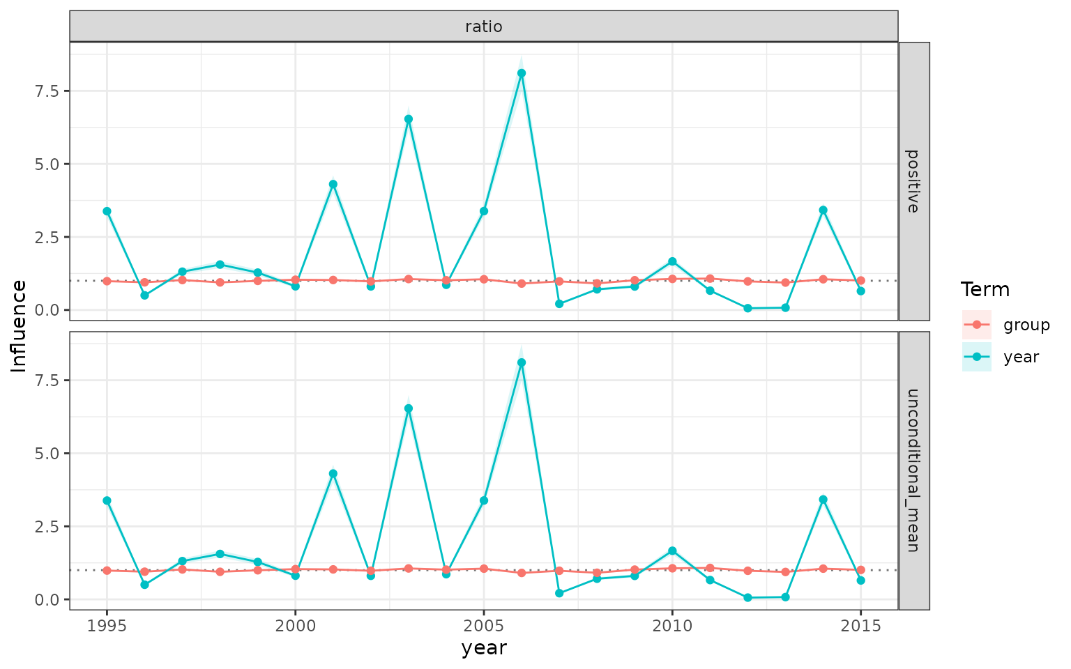

Positive, occurrence, and unconditional-mean influence from a brms hurdle-lognormal model.

Because this example has hu ~ 1, the probability of occurrence has no year-varying model term. Consequently, its unconditional year influence is the same as its positive-component year influence. A varying hurdle formula would allow both components to contribute.

glmmTMB hurdle example

For glmmTMB, the truncated conditional family and zero formula form a hurdle model. The package simulates the conditional and zero-formula coefficients jointly from the fitted covariance before combining them.

set.seed(31)
n <- 480
cpue <- data.frame(
  year = factor(rep(1:4, each = n / 4)),
  depth = rnorm(n)
)
positive_mean <- exp(0.5 + 0.1 * as.numeric(cpue$year) + 0.2 * cpue$depth)
zero_probability <- plogis(-0.8 + 0.15 * as.numeric(cpue$year))
cpue$catch <- ifelse(
  rbinom(n, 1, zero_probability),
  0,
  1 + rnbinom(n, mu = positive_mean, size = 2)
)

hurdle_fit <- glmmTMB::glmmTMB(
  catch ~ year + depth,
  ziformula = ~year,
  family = glmmTMB::truncated_nbinom2(),
  data = cpue
)
glmmTMB_hurdle <- influ(
  hurdle_fit,
  focus = "year",
  ndraws = 500,
  seed = 1
)
unique(glmmTMB_hurdle$influence$component)
#> [1] "positive"           "occurrence"         "unconditional_mean"

plot(glmmTMB_hurdle, type = "components")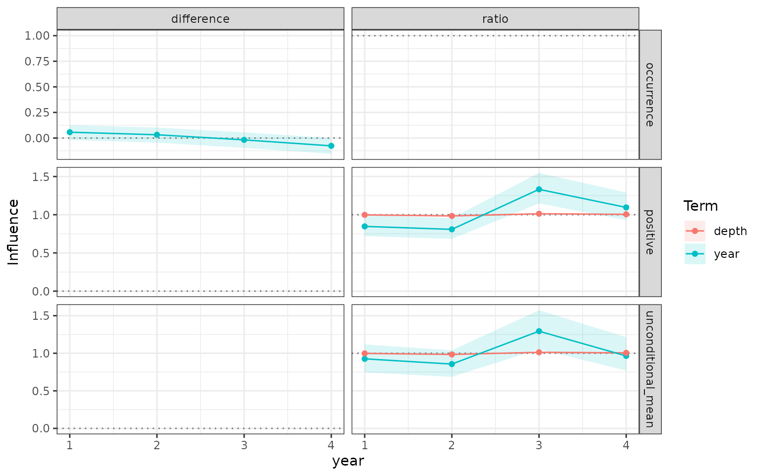

Positive, occurrence, and unconditional-mean influence from a glmmTMB hurdle model.

Zero-inflated Poisson and negative-binomial models follow the same pathway, with zero_probability and count labels replacing occurrence and positive.

When inspecting a term with plot(diagnostic, type = "cdi", term = ...), select one component at a time. The top panel centres that component’s effect on the same reference as its influence. Positive log-link and lognormal effects appear as ratios about one, whereas a logit occurrence or extra-zero effect remains in centred log-odds about zero. An increase in extra-zero log-odds has the opposite interpretation to an increase in occurrence log-odds. Neither is itself an unconditional catch multiplier; use the combined unconditional-mean influence to assess that quantity.

Dependence and memory

Component combination must be performed draw by draw, or with a joint covariance or precision calculation. Multiplying independently calculated marginal intervals is invalid because it loses dependence between the two linear predictors. influ2 therefore combines:

brms population-level components draw by draw from the joint posterior; and
glmmTMB fixed components draw by draw from their joint maximum-likelihood covariance; and
sdmTMB and tinyVAST latent fields draw by draw from their sparse joint precision matrices.

Only derived focus-by-term draws are retained when requested. The much larger observation-by-draw arrays are never stored.

For brms lognormal models, a constant residual-scale adjustment cancels from an influence ratio. Models in which sigma varies are rejected: they need a future joint location-and-scale calculation. brms lognormal location models also require their usual identity link. Mean-parameterised lognormal backends instead require a log link. In glmmTMB, varying data-scale dispersion does not invalidate log-link arithmetic-mean ratios, but its dispersion effects are not separately decomposed. Combined hurdle/zero-inflated diagnostics with offsets or exposure additions are also rejected until an offset-aware reference calculation is available.

Spatial delta models

sdmTMB and tinyVAST delta models expose occurrence and positive fixed effects and latent fields as named components. Their fixed effects are combined into an unconditional mean with joint covariance simulation. For example:

fit <- sdmTMB::sdmTMB(
  cpue ~ 0 + as.factor(year) + depth,
  data = cpue_data,
  mesh = mesh,
  time = "year",
  family = sdmTMB::delta_gamma()
)

diagnostic <- influ(fit, focus = "year")
plot(diagnostic, type = "components")

The combined delta mean also includes latent spatial and spatiotemporal fields. Both components are evaluated from the same sparse joint-precision draw before the unconditional mean is calculated, preserving posterior dependence rather than assembling independent marginal intervals. The motivation for this spatial extension follows Hsu et al. (2022).

References

Hsu, Jhen, Yi-Jay Chang, and Nicholas D. Ducharme-Barth. 2022. “Evaluation of the Influence of Spatial Treatments on Catch-Per-Unit-Effort Standardization: A Fishery Application and Simulation Study of Pacific Saury in the Northwestern Pacific Ocean.” Fisheries Research 255: 106440. https://doi.org/10.1016/j.fishres.2022.106440.