Model search

Search a scientific candidate set

search_cpue() searches a constrained set of model specifications. It protects the annual index term, exposure offsets, and essential random or spatial structure, then compares eligible candidates using a stated native criterion. The response can be CPUE, a count with an exposure offset, or another supported response: it need not be a catch.

This adds a different workflow to the existing interfaces:

• check_cpue() checks a model; its residual p-values are not term-removal rules.
• table_criterion() compares models that have already been fitted.
• influ_steps() and plot_step() show changes in annual contrasts along a prescribed sequence, rather than choosing that sequence.
• search_cpue() evaluates legal candidates and records a recommendation, together with its constraints, fitting evidence, and stopping reason.

One search uses one model backend, response definition, and family/link. A common interface across backends does not make AIC, conditional AIC, and LOOIC interchangeable. See Model comparison.

The starting model is a maximal candidate model, not necessarily a saturated model: it contains the terms we are prepared to consider. A saturated model has enough freedom to reproduce every observation and is not required here.

A worked glmmTMB lobster example

We use the same simulated lobster observations as the main article. Each observation represents one pot, so its expected response is lobsters per pot. The negative-binomial model accounts for extra-Poisson variation; month is a random intercept. Soak time is an ordinary predictor here, not an exposure offset or a likelihood weight.

data(lobsters_per_pot)
lobster_model <- glmmTMB::glmmTMB(
  lobsters ~ year + poly(depth, 3) + poly(soak, 3) + (1 | month),
  data = lobsters_per_pot, family = glmmTMB::nbinom2()
)

Inspect the plan before fitting

Without refit = TRUE, the function only prepares a plan. It does not fit models, calculate criteria, run MCMC, or simulate residuals. We nominate depth and soak as the only optional terms. The annual term and monthly random intercept remain in every candidate. A polynomial is one term block: all three basis coefficients move together.

search_plan <- search_cpue(
  lobster_model, year = "year", criterion = "BIC",
  optional = ~ poly(depth, 3) + poly(soak, 3), max_models = 16
)
search_plan
#> <influ_search> glmmTMB / BIC
#>   Mode: preflight only
#>   Protected terms: 2
#>   Evaluated candidates: 0
#>   Stop: preflight_only
knitr::kable(search_plan$terms[c("term", "protected", "reason")])

term	protected	reason
year	TRUE	annual predictor
poly(depth, 3)	FALSE	optional term block
poly(soak, 3)	FALSE	optional term block
1 | month	TRUE	essential random/spatial structure

criterion = "auto" uses native AIC for frequentist models and LOOIC for complete brms models. Here we explicitly choose BIC, which applies a stronger parameter penalty at this sample size. This is a choice of search criterion, not evidence that BIC is universally preferable for CPUE standardisation.

Run a bounded ordering and backward search

The default direction = c("order", "backward") first adds converged term blocks to the protected core, then considers backward deletions. During ordering, a block can enter even if the criterion worsens: the aim is an admissible maximal model. Backward moves must improve the criterion. The recommended fit is the best eligible model evaluated, which need not be the final path entry or a global optimum.

lobster_search <- search_cpue(
  lobster_model, year = "year", criterion = "BIC",
  optional = ~ poly(depth, 3) + poly(soak, 3),
  direction = c("order", "backward"), max_models = 16, refit = TRUE
)
lobster_search
#> <influ_search> glmmTMB / BIC
#>   Mode: native refitting
#>   Protected terms: 2
#>   Evaluated candidates: 4
#>   Stop: no_improving_legal_move
#>   Best evaluated: lobsters ~ (year) + (poly(depth, 3)) + (poly(soak, 3)) + (1 | month) (17925.27)
knitr::kable(
  lobster_search$candidates[c("candidate", "formula", "score", "status")],
  digits = 2, row.names = FALSE
)

candidate	formula	score	status
1	lobsters ~ (year) + (1 | month)	18195.44	eligible
2	lobsters ~ (year) + (poly(depth, 3)) + (1 | month)	18095.91	eligible
3	lobsters ~ (year) + (poly(soak, 3)) + (1 | month)	18023.16	eligible
4	lobsters ~ (year) + (poly(depth, 3)) + (poly(soak, 3)) + (1 | month)	17925.27	eligible

knitr::kable(lobster_search$path, digits = 2, row.names = FALSE)

step	phase	action	terms	candidate	score	improvement
0	order	start		1	18195.44	NA
1	order	add	poly(soak, 3)	3	18023.16	172.29
2	order	add	poly(depth, 3)	4	17925.27	97.89

This example retains both covariate blocks: automated searching need not delete something. Each distinct candidate is fitted at most once; revisiting it during backward checking reuses its recorded result. The original fit can also be reused when its specification and fitting controls match exactly.

plot(lobster_search)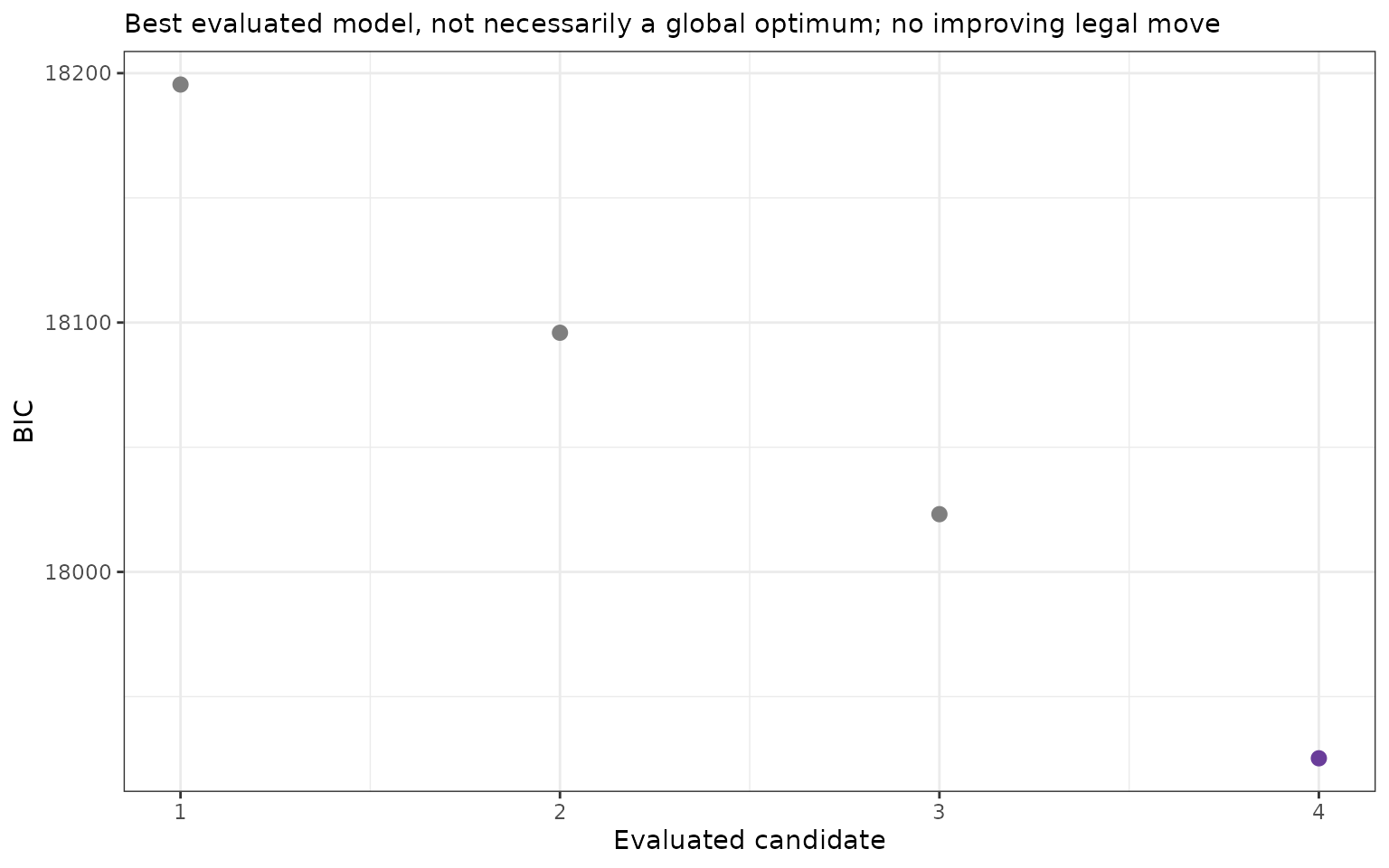

Native BIC values for eligible lobster glmmTMB candidates evaluated by the constrained search. The purple point identifies the best evaluated candidate. Year and the monthly random intercept are protected, and the depth and soak-time polynomial blocks are optional. Candidate numbers describe evaluation order, not a continuous model dimension. Lower BIC is preferred within this comparable candidate set; this display is not a residual goodness-of-fit test.

Retrieve the fit and calculate the CPUE index

selected_model() returns the retained native fitted model without refitting. It can go straight into the usual diagnostics and index interfaces. We use the same fixed reference profile as the CPUE indices article: median observed depth, a 24-hour soak, and monthly random effect zero. This zero-effect reference is not integration over the distribution of months.

recommended_model <- selected_model(lobster_search)
reference <- data.frame(depth = median(lobsters_per_pot$depth), soak = 24)
recommended_index <- cpue_index(
  recommended_model, year = "year", reference_data = reference,
  units = "lobsters per pot"
)
knitr::kable(index_table(recommended_index), digits = 3, row.names = FALSE)

Year	Mean	SD	CV	Q0.025	Q0.975	Method	Distribution	Link
2000	1.674	0.238	0.142	1.267	2.212	standardised	nbinom2	log
2001	1.744	0.247	0.142	1.321	2.303	standardised	nbinom2	log
2002	1.815	0.254	0.140	1.380	2.387	standardised	nbinom2	log
2003	1.387	0.189	0.136	1.062	1.812	standardised	nbinom2	log
2004	1.572	0.214	0.136	1.204	2.053	standardised	nbinom2	log
2005	1.310	0.185	0.141	0.993	1.729	standardised	nbinom2	log
2006	1.167	0.158	0.136	0.895	1.522	standardised	nbinom2	log
2007	1.184	0.161	0.136	0.907	1.545	standardised	nbinom2	log
2008	1.172	0.164	0.140	0.891	1.541	standardised	nbinom2	log
2009	1.123	0.157	0.140	0.853	1.477	standardised	nbinom2	log
2010	1.219	0.167	0.137	0.932	1.595	standardised	nbinom2	log
2011	1.379	0.189	0.137	1.055	1.803	standardised	nbinom2	log
2012	1.214	0.170	0.140	0.922	1.598	standardised	nbinom2	log
2013	1.372	0.187	0.136	1.051	1.792	standardised	nbinom2	log
2014	1.259	0.171	0.136	0.965	1.642	standardised	nbinom2	log
2015	1.067	0.146	0.137	0.816	1.395	standardised	nbinom2	log
2016	1.094	0.148	0.135	0.840	1.426	standardised	nbinom2	log
2017	1.118	0.153	0.137	0.855	1.462	standardised	nbinom2	log

plot_index(recommended_index)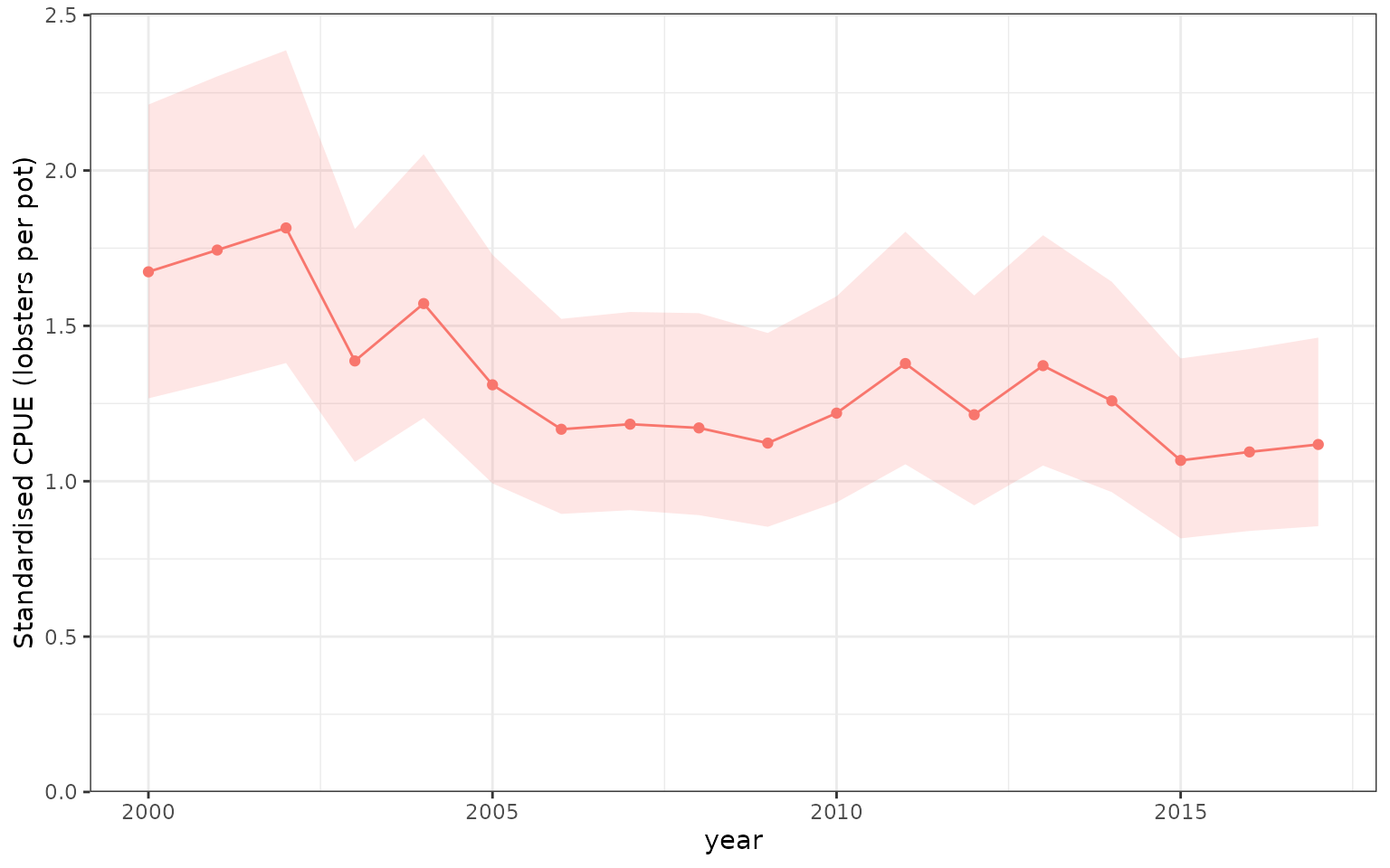

Standardised expected lobsters per pot from the recommended lobster glmmTMB model, at the fixed depth and soak-time reference profile and monthly random effect zero. The ribbon is a pointwise 95% confidence interval conditional on this fitted model. It does not include uncertainty from searching and choosing the model, and the index is not an area-integrated biomass estimate.

Search results retain the best native fit by default. keep_fits = "none" retains only the compact report; keep_fits = "all" can be useful for a small shortlist, but spatial or posterior model objects can be large. Printing, summarising, and plotting the saved search never repeat fits or residual simulations.

Compact retention limits the stored report and number of retained fits, not the native fitter’s peak RAM. Native LOO calculations for brms and spatial Hessian calculations can still require substantial temporary memory.

Explicitly search a non-essential random term

Random effects are protected by default. To ask whether a particular random term is needed, nominate that whole term explicitly. Here we examine the monthly intercept while holding the annual, depth, and soak specifications unchanged. This is a second scientific question, not an automatic licence to discard all random effects.

month_search <- search_cpue(
  lobster_model, year = "year", optional = "1 | month",
  direction = "backward", criterion = "BIC", max_models = 2, refit = TRUE
)
knitr::kable(
  month_search$candidates[c("candidate", "formula", "score", "status")],
  digits = 2, row.names = FALSE
)

candidate	formula	score	status
1	lobsters ~ (year) + (poly(depth, 3)) + (poly(soak, 3)) + (1 | month)	17925.27	eligible
2	lobsters ~ (year) + (poly(depth, 3)) + (poly(soak, 3))	18338.25	eligible

The coefficients and dispersion parameters are re-estimated in the reduced fit. Protecting a structure means keeping its specification, not fixing its numerical estimates. A BIC recommendation does not establish that removing a process is scientifically sensible; inspect uncertainty, residual structure, and the resulting index separately.

Annual interactions, exposure, and other backends

For annual-by-season coding such as fyear:season, explicitly protect that annual block. This unexecuted example illustrates a CRA-style specification; the data and fitted object are supplied by the analyst, not by this vignette.

plan <- search_cpue(
  seasonal_model, year = "fyear", include = ~ fyear:season,
  optional = ~ poly(depth, 3) + poly(soak, 3), criterion = "BIC"
)
result <- search_cpue(
  seasonal_model, year = "fyear", include = ~ fyear:season,
  optional = ~ poly(depth, 3) + poly(soak, 3), criterion = "BIC",
  refit = TRUE, max_models = 16
)

Offsets, fitted rows, likelihood weights, binomial trial counts, and the response definition must agree across candidates. For counts fitted with offset(log(exposure)), that offset remains present. If the response is already CPUE, adding an exposure offset again is not an automatic default. Searches do not silently change the data subset as terms are removed.

The same interface accepts GLM, mgcv GAM, lme4, glmmTMB, complete brms, sdmTMB, and univariate tinyVAST models, subject to supported formula and likelihood contracts. Backend-specific restrictions are explicit:

• Smooths are term blocks; essential random or multidimensional smooths remain protected unless deliberately nominated. Existing interaction hierarchy is preserved without inventing main effects for intentional interaction-only annual coding.
• Gaussian mixed models fitted with REML are refitted with ML when searching fixed effects, and that conversion is recorded.
• glmmTMB zero-inflation and dispersion formulas remain fixed in this increment. The search changes its main conditional formula only.
• A joint sdmTMB delta search needs component = "occurrence" or "positive". The other formula, shared spatial domain, and process settings remain fixed; it is not simultaneous selection of both components.
• Spatial fields, spatiotemporal processes, and meshes are not automatically switched on or off. Compare deliberately fitted process alternatives using table_criterion() and the diagnostic interfaces.
• Explicit positional parameter maps are not automatically remapped when terms change. For mapped TMB fits, fit named candidate specifications separately, then use table_criterion(). Saved sdmTMB process formulas and binomial trial counts remain fixed, even if variables in the original call have since changed.
• brms searches require new MCMC fits for changed models. Use an explicit candidate budget and native sampling controls; incomplete fits or unreliable LOO estimates cannot win. This vignette does not run MCMC.

# Preflight reports only: no refits or new criteria.
search_cpue(gam_model, year = "year", optional = ~ s(depth))
search_cpue(spatial_model, year = "year", optional = ~ depth)
search_cpue(delta_model, year = "year", component = "positive",
  optional = ~ depth)
search_cpue(bayesian_model, year = "year", optional = ~ depth,
  max_models = 6)

What the search can and cannot establish

The report includes every evaluated specification, numerical status, warnings, criterion, and stopping reason. Failed or incomparable candidates remain visible but are ineligible. max_models counts distinct attempts, including failures and a reused original fit. Reaching the limit leaves a bounded result, not a claim that the search finished exploring the candidate set.

The function is a fresh, backend-aware controller inspired by the ordering and elimination workflow in buildmer, rather than a call to buildmer::buildglmmTMB() under a different name. Small native ML tests compare forward and backward BIC selections with buildmer. This does not imply identical paths, tie handling, random-effect eligibility rules, or finalisation for every model. The glmmTMB model-evaluation vignette also illustrates stats::drop1() and MuMIn::dredge() workflows. Their ideas of protected terms, interaction hierarchy, and comparable observations are useful, but unrestricted all-subsets fitting is not the default here.

Native AIC is the frequentist default; BIC is optional. Native conditional AIC is available only where supported and validated, not through an invented generic mixed-model correction. Complete brms candidates use LOOIC rather than AIC. Comparisons across inappropriate likelihood targets, priors, response supports, or observations are rejected rather than ranked together.

Finally, the best observation-model score is not proof that the CPUE index tracks abundance. Searching can favour a spurious specification, and ordinary intervals after selection understate the full uncertainty if model-selection uncertainty is ignored. Retain a scientifically justified candidate set, check the shortlist with check_cpue(), and examine index sensitivity using plot_compare() or deliberately chosen step sequences before accepting a model for assessment.