Calculate compact simulation-based residual diagnostics

Calculate once, then use plot.influ_residuals() for a four-panel overview: a normal-score rank Q-Q plot, residuals against the predictive mean, residuals by year, and a response-adaptive calibration or distribution panel.

Usage

influ_residuals(
  model,
  data = NULL,
  year = NULL,
  nsim = 250L,
  batch_size = 25L,
  seed = 1L,
  grid_size = 201L,
  level = 0.95,
  component = c("auto", "combined", "encounter", "positive"),
  calibration_bins = 10L,
  calibration_min_n = 20L,
  calibration_groups = NULL,
  trial_counts = NULL,
  groups = NULL,
  conditioning = "backend_default"
)

# S3 method for class 'influ_residuals'
print(x, ...)

Arguments

model: A fitted GLM, mgcv GAM, glmmTMB, brmsfit, sdmTMB, or single-response tinyVAST model. No model is fitted by this function.
data: Original model data, retaining original row names. Usually not needed; supply it if a transformed time term hides the raw year column.
year: Name of the time column. By default, recognise year/fishing-year names in the formula, then native time metadata or a time-named term, then the first single-variable formula term (with a warning). Ambiguous choices require an explicit override. No arbitrary grouping is selected.
nsim: Number of complete response simulations, at least 20.
batch_size: Maximum number of simulations requested in each batch.
seed: Integer random seed. The caller's random-number state is restored.
grid_size: Approximate number of ECDF grid points, at least 20.
level: Pointwise predictive interval coverage for ECDFs, and nominal independent-uniform reference coverage for the Q-Q panel.
component: Response to diagnose: "auto" retains a joint model's "combined" response; "encounter" selects presence in supported hurdle models, and "positive" selects native sdmTMB component-2 simulations at rows with observed positive catch. Separate encounter/positive fits may also be labelled explicitly. Unsupported component extraction fails.
calibration_bins: Requested number of roughly equal-observation-count probability bins. Defaults to 10; ties are never split. Near ties within 1e-8 are kept together, and under-supported bins are merged.
calibration_min_n: Minimum observation count per probability bin, default 20. Smaller datasets remain a single flagged sparse bin. Scientific groups below this size remain visible but have no predictive envelope.
calibration_groups: Optional character vector of original-data columns defining a joint scientific grouping, e.g. c("year", "target"). These columns must not be defined from the outcome. Supply data if necessary.
trial_counts: For weighted one-column binomial GLM/GAM/glmmTMB fits, the name of the known trial-count column in data. It must equal the fitted trial weights. Arbitrary case weights are not treated as trials. Two-column success/failure responses need no override.
groups: Optional names of original-data grouping columns to retain for plot_grouped_residuals(). Specify these independently of the response. Only these columns, not the complete model data, are stored.
conditioning: Simulation target. "backend_default" preserves existing behaviour: "fitted" for GLM/GAM/sdmTMB/tinyVAST, "new_effects" for glmmTMB, and "posterior_predictive" for brms. Explicit alternatives are "fitted" for glmmTMB, "conditional_draw" for sdmTMB/tinyVAST, and "new_effects" for sdmTMB. Unsupported combinations fail, not fall back. See the conditioning section below before comparing model diagnostics.
x: An `influ_residuals` object.
...: Reserved for future methods; currently unused.

Value

An S3 influ_residuals object containing observation-level ranks, normal scores, predictive means, year labels, Q-Q reference coordinates, compact ECDF summaries, and explicit calculation metadata.

Details

Each simulation is a joint response vector, preserving the native method's within-draw dependence. For observation $i$, let $L_i$ count simulated responses below the observation and $E_i$ count ties. The randomised finite-simulation rank is $(L_i + U_i(E_i + 1))/(B + 1)$, with independent uniform $U_i$. Its normal score is a simulation-based quantile residual, not a Pearson residual or an exact analytic PIT. Randomisation includes zeros and other atoms without adding arbitrary noise to catches. Increase nsim and inspect seed sensitivity for important conclusions.

GLMs and GAMs simulate observation error at fitted parameters, including fitted smooths. glmmTMB uses its native simulation of new random effects. sdmTMB and tinyVAST use type = "mle-eb": observation error conditional on fitted latent effects. brms uses joint posterior predictive draws, including existing group effects. These are different diagnostic targets, not interchangeable uncertainty estimates. The predictive mean on the horizontal axis is estimated from these same simulations, so it matches their conditioning rather than mixing in differently conditioned fitted values. No refitting, MCMC, or leave-one-out calculation is performed.

The Q-Q band is an independent-uniform reference, not a calibrated goodness-of-fit test for estimated, hierarchical, spatial, or Bayesian models. Posterior predictive ranks reuse the observations and need not be uniform. ECDF bands are pointwise simulated-response bands, not simultaneous confidence bands. By default, zero-inflated and delta simulations describe the combined response, not either component separately. Censored, multivariate, quasi-family, and non-binomial weighted fits are not supported. Native simulation failures are reported, not replaced by another family. A positive-component check needs its own fitted component and matching observations, or an explicit native component diagnostic; do not relabel or subset the combined-response overview as a positive-component check.

Bernoulli calibration uses native fitted probabilities, including fitted effects, separately from the simulation mean used in the first three panels. brms averages expected probabilities over the same posterior draw identities used for simulation. Bins are fixed before simulation. Whole simulated response vectors are reduced to proportions within those bins; their pointwise predictive envelopes are not confidence intervals for an underlying calibration curve or calibrated goodness-of-fit tests. In particular, glmmTMB simulations redraw random effects although binning uses fitted conditional probabilities, so the envelope need not centre on the identity line. Dependence is only that represented by the native simulator; no extra vessel or temporal dependence is added. Fitted-data calibration, including grouped checks, is exploratory. Matching overall or annual means may follow from fitted intercept/year effects and does not validate a model.

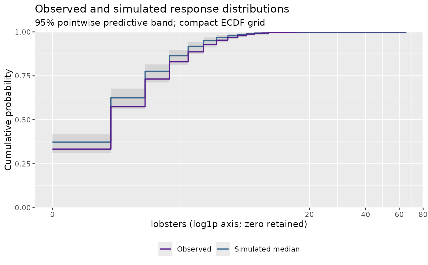
The object retains neither the fitted model nor an observation-by-simulation matrix. Working storage includes an observation-by-batch matrix and a grid-by-simulation matrix, plus compact bin/group simulation summaries. Native backends may allocate additional memory. The ECDF grid spans observations and the first simulation batch; it is deliberately compact, not an exact representation of every simulated jump. For binomial GLMs and glmmTMB, responses are success counts (including proportion responses with integer trial weights).

Conditioning

"fitted" holds fitted parameters and latent effects fixed while simulating observation variation. "conditional_draw" holds fixed parameters at their estimates, draws one joint latent-effect vector from the native TMB Gaussian conditional approximation, and reuses it for every response simulation and batch. It requires a converged, unprofiled ML (not REML) fit with latent effects and a positive-definite Hessian. The sparse factorisation and one parameter vector are prepared once; neither the draw nor the response matrix is retained. This is not MCMC or integration over fixed-parameter uncertainty.

"new_effects" regenerates latent processes at fitted distribution parameters: glmmTMB uses its native random-effect simulation, and sdmTMB uses the same controls as simulate(..., re_form = NA) (fitted smooths remain fixed). "posterior_predictive" retains brms joint posterior uncertainty, including existing group effects. These are different questions, not interchangeable ways to obtain uniformly distributed fitted-data ranks.

Explicit glmmTMB "fitted" and the new spatial schemes use an independent native objective; the user's fitted object is not altered. For these schemes, per-replicate seeds and a shared latent draw make observation-level results invariant to batch_size. The compact response-ECDF grid still depends on the first batch. Existing default simulation/RNG behaviour is unchanged. Sampled-field binomial/encounter probabilities use the same latent vector. New-effect calibration retains fitted conditional probability bins, so the predictive envelope need not centre on the identity line. Check metadata$scheme, metadata$conditioning, and metadata$prediction_type. Native versions and support can differ; no term-by-term conditioning control or automatic MCMC, marginal integration, or new-group brms prediction is added.

Examples

if (requireNamespace("glmmTMB", quietly = TRUE)) {
data(lobsters_per_pot)
fit <- glmmTMB::glmmTMB(
  lobsters ~ year + poly(depth, 3) + poly(soak, 3) + (1 | month),
  family = glmmTMB::nbinom2(), data = lobsters_per_pot)
checks <- influ_residuals(fit, nsim = 50, seed = 42)
checks
plot(checks)
plot(checks, type = "qq")
plot(checks, type = "distribution", response_scale = "log1p")
}