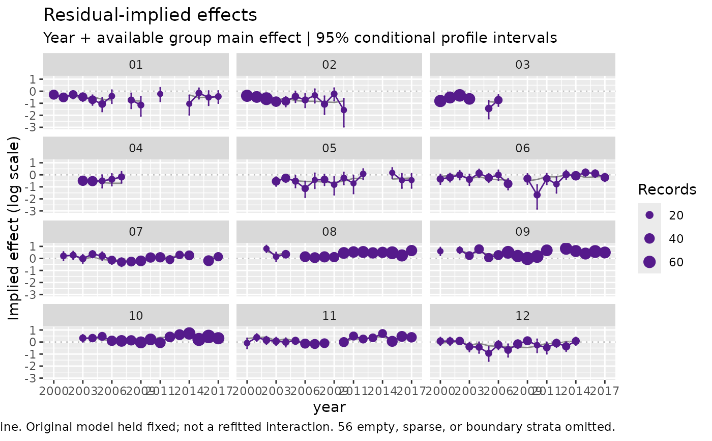
Calculate residual-implied effects by year and group

Estimate a local effect-scale adjustment while holding the supplied model fixed, then add it to a centred year (and optionally group) contribution. These exploratory trajectories are not refitted interactions or regional abundance indices. Calculate once and plot the compact result repeatedly.

Usage

implied_effects(
  model,
  data = NULL,
  year = NULL,
  groups = "area",
  method = c("likelihood", "traditional"),
  baseline = c("year_group", "year"),
  min_n = 10L,
  level = 0.95,
  interval = c("auto", "descriptive", "none"),
  traditional_scale = c("log_response", "standardised", "standardized")
)

# S3 method for class 'influ_implied'
print(x, ...)

# S3 method for class 'influ_implied'
as.data.frame(x, row.names = NULL, optional = FALSE, ...)

Arguments

model: A retained lm, GLM, mgcv GAM, or ML glmmTMB fit. This first implementation supports Gaussian identity-link models (including an explicitly logged response), Poisson, NB2, and Gamma log-link models. Other families, backends, joint models, non-unit case weights, and year interactions fail explicitly rather than substitute another calculation.
data: Original model data with original row names, if needed to recover the year or grouping column. Values are checked against the fit.
year: Time column; NULL uses the usual automatic detection.
groups: One original-data grouping column, not defined by the response.
method: "likelihood" (default) estimates a one-parameter conditional likelihood shift per stratum. "traditional" adds mean log-scale residuals for a Gaussian model of log(response); see traditional_scale.
baseline: "year_group" adds the centred, fixed main contributions of year and group, where the group main effect is present. "year" adds only the year contribution. Terms are centred over all fitted observations, not separately within panels. An additive fixed year term is required. Random effects and smooths remain in fitted predictions, not the baseline.
min_n: Minimum records in a year-by-group stratum. Sparse and empty strata remain in the table with an explicit status, but are not plotted.
level: Conditional profile-likelihood interval coverage; default 0.95.
interval: "auto" uses profile-likelihood intervals for the new method, or mean +/- one descriptive SE for traditional calculations. "descriptive" uses SD/sqrt(n) of log-scale residuals for either method in constant-variance Gaussian log-response models. "none" omits bars.
traditional_scale: "log_response" uses ordinary log-response residuals. "standardised" (or "standardized") reproduces the historical analyser GLM convention: native rstandard() residuals, globally centred, added to term contributions. This latter display mixes scales, is retained only for comparison, and is restricted to plain Gaussian log-response GLMs.
x: An `influ_implied` result.
...: Unused for printing and table extraction.
row.names: Optional row names for the extracted table.
optional: Passed to [as.data.frame()].

Value

A compact influ_implied object with a stratum table and explicit metadata. No fitted model or observation-level arrays are retained.

Details

For each stratum, the likelihood method replaces its original linear predictor eta by eta + delta, holding all other parameters, fitted random effects, smooths, offsets, and dispersion values fixed. Gaussian shifts are precision-weighted mean response residuals. With constant variance and an explicitly logged response this equals the traditional mean log-response residual. NB2 uses the fitted size parameter and its log likelihood, not a mean of Pearson or PIT residuals. Gamma(log) uses the native fitted scale phi (variance = phi * mean^2), with shape = 1/phi. Its shift is log(sum(shape * response / fitted_mean) / sum(shape)), or log(mean(response / fitted_mean)) for constant scale. GAMs retain sig2, GLMs use summary(model)$dispersion, and glmmTMB uses squared native dispersion predictions. No shape is re-estimated. Gamma responses must be strictly positive; other Gamma links and joint delta models are not automatically reinterpreted as Gamma(log) fits.

Automatic intervals condition on the whole original fit. They omit uncertainty in its parameters, latent effects, and baseline, and do not account for residual dependence. They are neither full interaction confidence intervals nor Bayesian credible intervals. Descriptive bars are one SE, not intervals with level coverage. No MCMC, full-model refit, posterior averaging, response simulation, or area integration is done.

For all-zero count strata the optimum is delta = -Inf. These boundary results are retained and flagged, not replaced with a pseudocount or a finite correction. Their points/bars are omitted from the plot. Empty and sparse cells, and missing numeric years, break trajectories. Existing influ_residuals objects do not contain the native likelihood needed here: use plot_grouped_residuals() for their zero-centred grouped PIT summaries.

Directly parameterised lognormal families are not supported in this first increment. In particular, glmmTMB parameterises lognormal mean and SD on the response scale; holding that SD fixed is not the same as a constant log-SD shift. Use a Gaussian model of log(response) for the demonstrated equivalence, not an automatic reinterpretation of another fitted family.

References

The historical analyser Diagnoser implementation adds selected fitted terms to globally centred rstandard() residuals for GLMs: https://github.com/trophia/analyser/blob/master/R/diagnoser.r. Ordinary log-response residuals are a separate, explicitly named convention.

Examples

data(lobsters_per_pot)
fit <- glm(lobsters ~ year + month + depth, family = poisson(),
  data = lobsters_per_pot)
result <- implied_effects(fit, groups = "month")
head(as.data.frame(result))
#>   level group  n   baseline  adjustment   estimate std_error      lower
#> 1  2000    01 36 -0.4426083  0.15756268 -0.2850456 0.1428571 -0.5787395
#> 2  2001    01 34 -0.3784734 -0.13844015 -0.5169135 0.1601282 -0.8480707
#> 3  2002    01 26 -0.3201948  0.04453766 -0.2756571 0.1643990 -0.6161470
#> 4  2003    01 29 -0.6410748  0.16243930 -0.4786355 0.1714986 -0.8347003
#> 5  2004    01 25 -0.4674742 -0.24329095 -0.7107652 0.2085144 -1.1492843
#> 6  2005    01 19 -0.6696967 -0.39160822 -1.0613050 0.2886751 -1.6858731
#>         upper status
#> 1 -0.01752950     ok
#> 2 -0.21866108     ok
#> 3  0.03014534     ok
#> 4 -0.16032639     ok
#> 5 -0.32812550     ok
#> 6 -0.54419913     ok
plot(result)