Introduction
This article records supporting implementation diagnostics for developers. They are not fitting instructions or assessment results.
Note
The calculations use the package’s conditional API smoke fixture. Only CPUE and gene-tag catchability were re-estimated in that fixture; it is not a scientific stock-assessment fit.
Unfished flat-TRO diagnostic
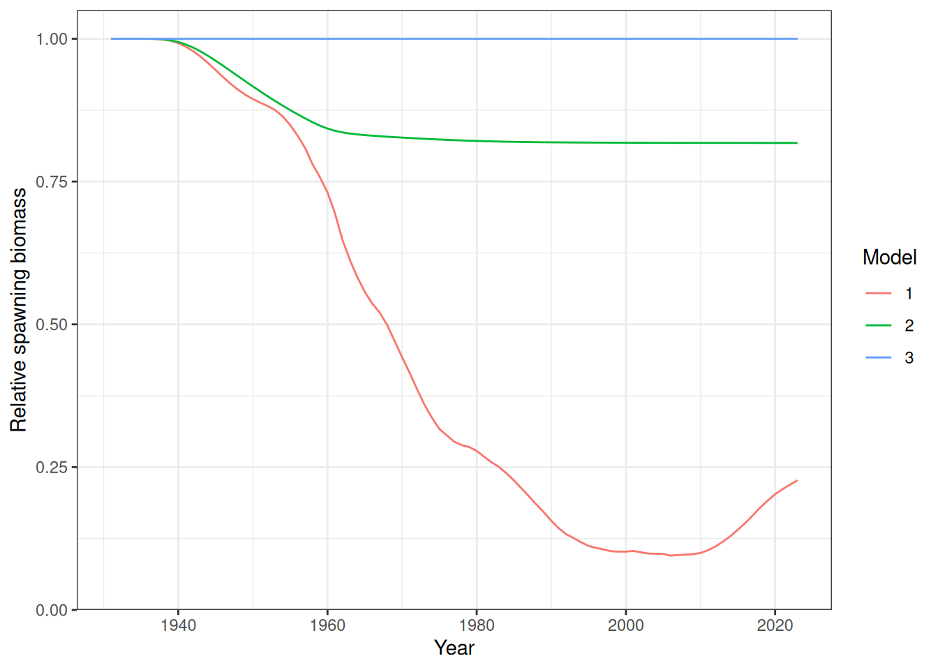
To get a flat total reproductive output trend we need to set catch to zero. Some of the time-varying inputs also need to be set so that they are the same as the first model year in all years. These time-varying inputs include mean length (length_mu_ysa) and phi_ya. The dl_l integration weights are common across years and ages.
Loading required package: RTMB
Loading required package: RTMBdist
Attaching package: 'RTMBdist'
The following objects are masked from 'package:RTMB':

    dbeta, dnbinom2
The following objects are masked from 'package:stats':

    dbeta, plnorm, pt
── Attaching core tidyverse packages ──────────────────────── tidyverse 2.0.0 ──
✔ dplyr     1.2.1     ✔ readr     2.2.0
✔ forcats   1.0.1     ✔ stringr   1.6.0
✔ ggplot2   4.0.3     ✔ tibble    3.3.1
✔ lubridate 1.9.5     ✔ tidyr     1.3.2
✔ purrr     1.2.2
── Conflicts ────────────────────────────────────────── tidyverse_conflicts() ──
✖ dplyr::filter() masks stats::filter()
✖ dplyr::lag()    masks stats::lag()
ℹ Use the conflicted package (<http://conflicted.r-lib.org/>) to force all conflicts to become errors
theme_set(theme_bw())

fixture <- new.env(parent = emptyenv())
load(system.file("extdata", "opt.rda", package = "sbt"), envir = fixture)
fit <- sbt_fit(fixture$data)
fit <- sbt_add_parameters(fit, parameters = fixture$parameters)
fit <- sbt_add_map(fit, map = fixture$map)
fit <- sbt_add_bounds(fit, bounds = fixture$bounds)
fit <- sbt_build_object(fit)
obj <- sbt_obj(fit)
invisible(obj$fn(fixture$opt$par))
data <- fit$data
parameters <- fixture$parameters
map <- fixture$map

all(data$length_mu_ysa[1,,] == data$length_mu_ysa[92,,])
all(obj$report()$phi_ya[1,] == obj$report()$phi_ya[92,])
data2 <- data
data2$catch_obs_ysf[] <- 0
data2$tag_switch <- 0
for (y in seq_len(data$n_year)[-1L]) {
  data2$length_mu_ysa[y,,] <- data$length_mu_ysa[1,,]
}
We also need to set all recruitment deviates (par_rdev_y) to zero.
par2 <- parameters
par2$par_rdev_y[] <- 0
obj2 <- RTMB::MakeADFun(
  func = cmb(sbt_model, data2),
  parameters = par2,
  map = map
)
The standard deviation for recruitment deviates (par_log_sigma_r) must also be set effectively to zero to get a flat line. The smallest positive finite double is used so the log-scale parameter remains finite.
par3 <- par2
par3$par_log_sigma_r <- log(.Machine$double.xmin)
obj3 <- RTMB::MakeADFun(
  func = cmb(sbt_model, data2),
  parameters = par3,
  map = map
)

plot_biomass_spawning(data_list = list(data, data2, data2),
                      object_list = list(obj, obj2, obj3))
Analytic Hessian
Try the analytic Hessian.
# he <- obj$he()
# he_inv <- solve(he)
# he_ch <- chol(he)
# ev <- eigen(he)
# range(ev$values)
Calculate standard deviations of all model parameters, including non-linear functions of random effects and parameters specified through the ADREPORT() macro from the user template: