library(kableExtra)
library(tidyverse)
library(sbt)
library(reshape2)
library(SparseNUTS)
library(abind)
library(microbenchmark)

theme_set(theme_bw())

load(system.file("extdata", "opt.rda", package = "sbt"))
load(system.file("extdata", "mcmc.rda", package = "sbt"))
obj <- MakeADFun(func = cmb(sbt_model, data), parameters = parameters, map = map)
invisible(obj$fn(opt$par))Load packages and inputs
Load the MLE and MCMC done previously.
Simulation
Simulation can be done for any data set in the model that is passed through the RTMB function OBS [@Kristensen2016, @Kristensen2024]. For example, in the file R/likelihoods.R, the function get_cpue_like includes the code:
cpue_log_obs <- log(cpue_obs)
cpue_log_obs <- OBS(cpue_log_obs)
lp <- -dnorm(x = cpue_log_obs, mean = cpue_log_pred, sd = cpue_sig, log = TRUE)
This allows a call to obj$simulate()$cpue_log_obs. For example (see Figure 1):
# obj$simulate()$cpue_log_obs
# obj$simulate()$troll_log_obs
# obj$simulate()$aerial_log_obs
# obj$simulate()$gt_nrec
# obj$simulate()$hsp_nK
# obj$simulate()$pop_nP
plot(data$cpue_year, data$cpue_obs, col = 2)
for (i in 1:10) lines(data$cpue_year, exp(obj$simulate()$cpue_log_obs))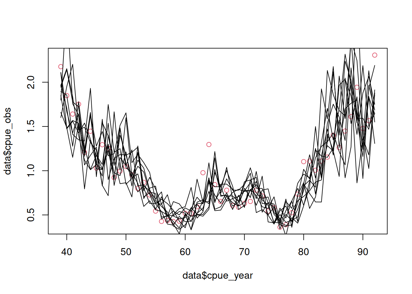
Data sets for which simulation is available include:
cpue_log_obstroll_log_obsaerial_log_obsgt_nrechsp_nKpop_nP
But not:
af_obslf_obscpue_lfs
Simulation is also required for calculating OSA residuals and to use the RTMB function checkConsistency. Unfortunately, the checkConsistency does not work yet because not all data types are defined using densities that have simulation support within the model (i.e., the AFs and LFs).
# chk <- checkConsistency(obj = obj, hessian = TRUE, estimate = TRUE, n = 100,
#                         observation.name  = "cpue_log_obs")
# chk
# s <- summary(chk)
# s
# s$marginal$p.value
Projection
Projections can be based on MLE or MCMC.
# iters <- sample(x = 1:2000, size = 1000)
iters <- 1:2000 # define the exact iterations you want to use
n_iter <- length(iters)
n_proj <- 13
proj_years <- (data$last_yr - 1):(data$last_yr + n_proj)
n_proj <- length(proj_years)
range(proj_years)
[1] 2021 2035Recruitment
First we explore the recruitment deviates estimated by the model. The Augmented Dickey-Fuller (ADF) test was applied to the recruitment deviates series, yielding a test statistic of -3.4661 with a lag order of 4. The p-value of approximately 0.049 indicates that, at the 5% significance level, we can reject the null hypothesis of a unit root, supporting the alternative hypothesis that the series is stationary. This suggests that the rdevs time series does not exhibit non-stationary behavior, such as trends or random walks, making it suitable for modeling with processes like ARIMA without requiring differencing to achieve stationarity.
rdevs <- obj$report()$rdev_y
# tseries::adf.test(rdevs)
Note that there is evidence for up to AR2
acf(rdevs)
# pacf(rdevs)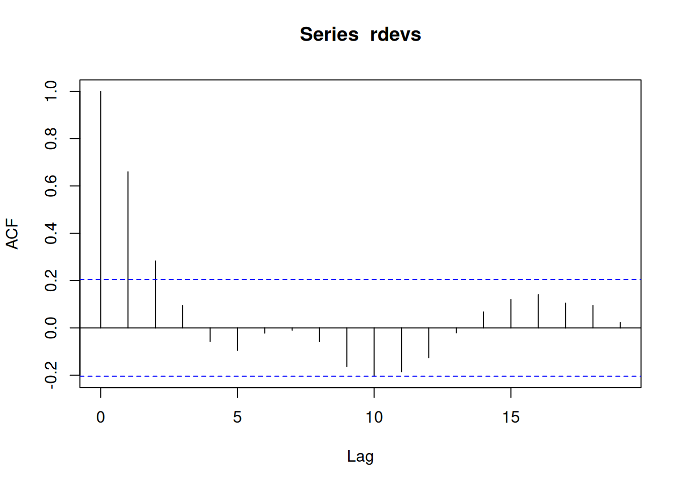
Must set method = "mle".
# auto.arima(rdevs)
ar(rdevs, order.max = 5)
Call:
ar(x = rdevs, order.max = 5)

Coefficients:
      1        2
 0.8382  -0.2702

Order selected 2  sigma^2 estimated as  0.0715
ar(rdevs, order.max = 5, method = "mle")
Call:
ar(x = rdevs, order.max = 5, method = "mle")

Coefficients:
      1        2
 0.8324  -0.2618

Order selected 2  sigma^2 estimated as  0.06879
Call:
arima(x = rdevs, order = c(2, 0, 0))
Coefficients:
ar1 ar2 intercept
0.8324 -0.2618 -0.0073
s.e. 0.0999 0.1010 0.0632
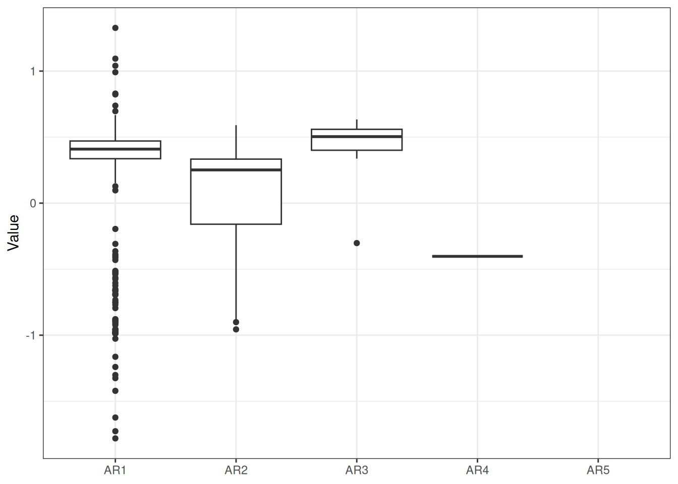
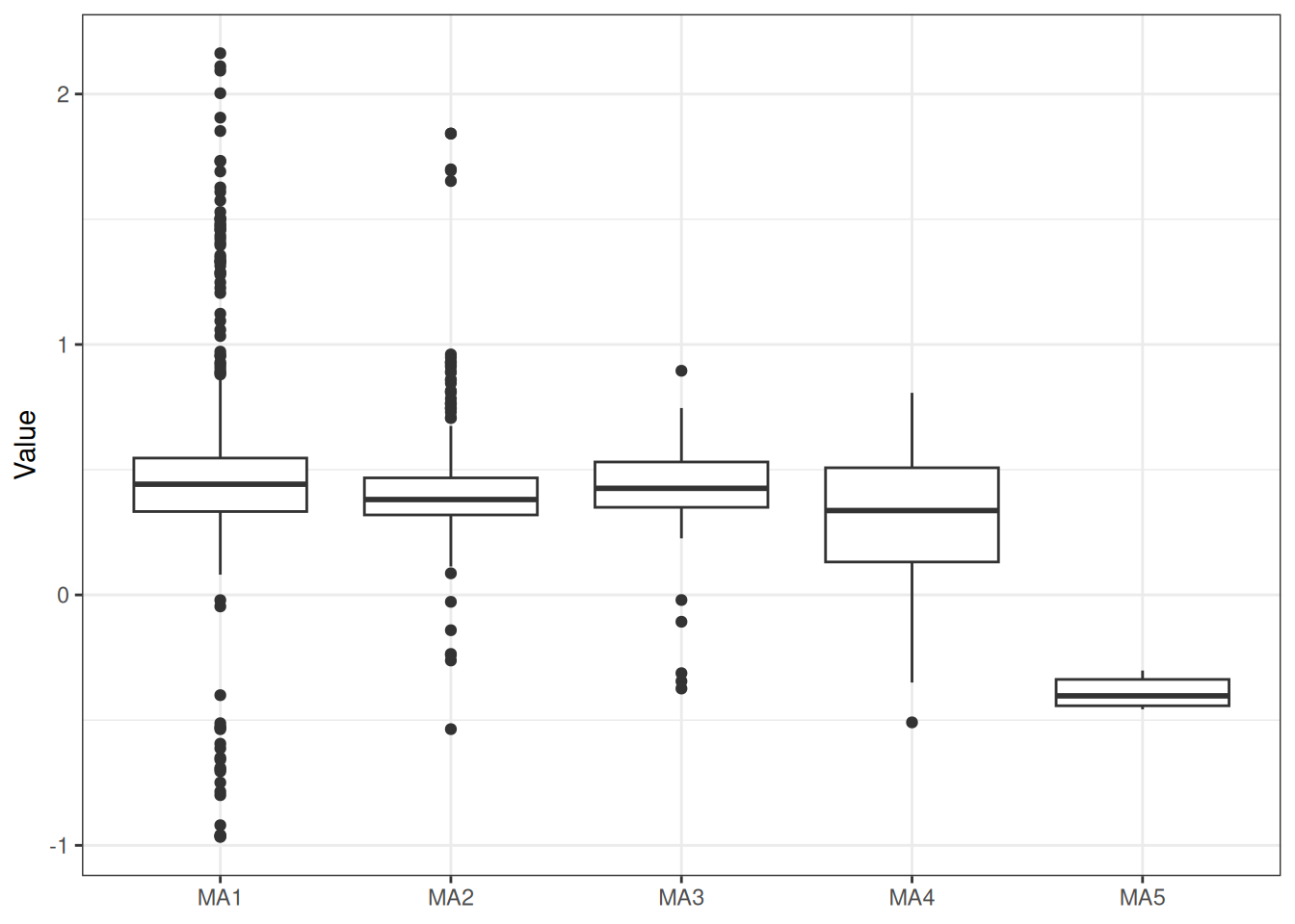
sigma^2 estimated as 0.06879: log likelihood = -7.77, aic = 23.54Recruitment projections can be based on an MLE fit or MCMC using the project_rec_devs function. These projections can be done using Autoregressive Integrated Moving Average (ARIMA) models by setting option = "ARIMA". Note that I am using bootstrap = TRUE. The samp_years input defines the range of years that we will use to model future recruitment deviates. We can then begin the projection before or after the last OM year, for example, if the last model year is 2022 and we begin the projection in 2021, then the final two recruitment deviates will be overwritten in our projection. Results are shown for MLE without ARIMA (Figure 3), MCMC without ARIMA (Figure 4), and MCMC with ARIMA (Figure 5). A comparison of all projections is shown in Figure 6. ARIMA order summaries are shown in Figure 7, with AR parameters in Figure 8 and MA parameters in Figure 9.
proj_rdev_MLE <- project_rec_devs(
  data = data, obj = obj, mcmc = NULL, first_yr = 2021, last_yr = 2035,
  samp_years = 1931:2020, iters = iters, option = "AR1"
)
proj_rdev_AR1 <- project_rec_devs(
  data = data, obj = obj, mcmc = mcmc, first_yr = 2021, last_yr = 2035,
  samp_years = 1931:2020, iters = iters, option = "AR1"
)
proj_rdev_ARIMA <- project_rec_devs(
  data = data, obj = obj, mcmc = mcmc, first_yr = 2021, last_yr = 2035,
  samp_years = 1931:2020, iters = iters, option = "auto"
)
plot_rec_devs(data = data, object = obj, posterior = mcmc, proj = proj_rdev_MLE)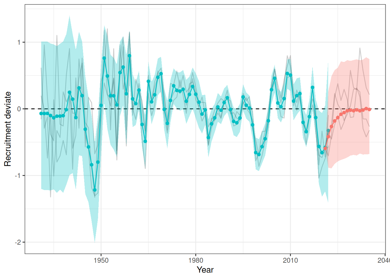
plot_rec_devs(data = data, object = obj, posterior = mcmc, proj = proj_rdev_AR1)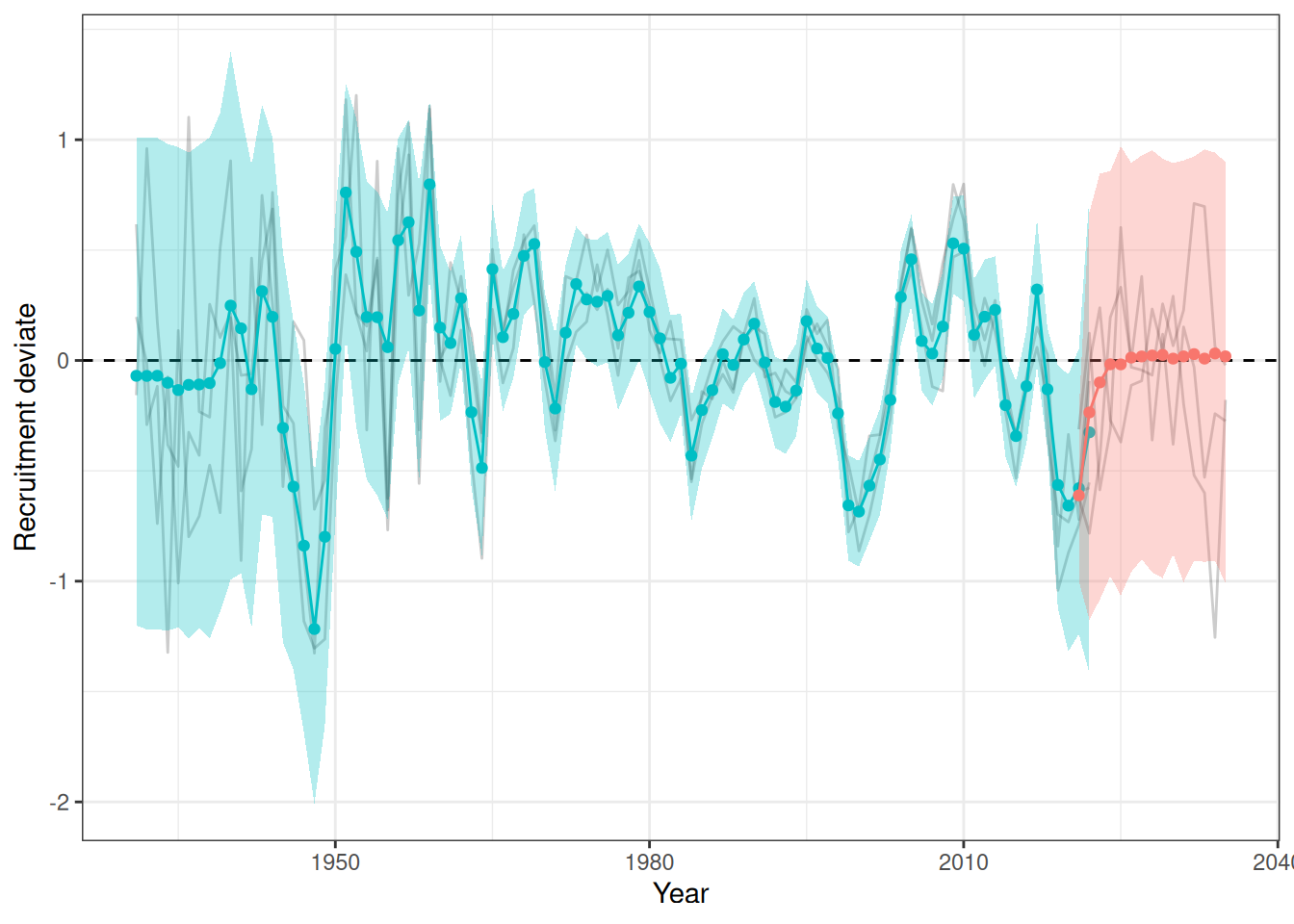
plot_rec_devs(data = data, object = obj, posterior = mcmc, proj = proj_rdev_ARIMA)
df <- bind_rows(
  melt(proj_rdev_MLE$proj_rdev_y) %>% mutate(Projection = "MLE AR1"),
  melt(proj_rdev_AR1$proj_rdev_y) %>% mutate(Projection = "MCMC AR1"),
  melt(proj_rdev_ARIMA$proj_rdev_y) %>% mutate(Projection = "MCMC ARIMA"))

ggplot(data = df, aes(x = year, y = value, fill = Projection, color = Projection)) +
  geom_hline(yintercept = 0, linetype = "dashed") +
  stat_summary(geom = "point", fun = median) +
  stat_summary(geom = "line", fun = median) +
  stat_summary(geom = "ribbon", fun.data = ~ data.frame(ymin = quantile(.x, 0.025), ymax = quantile(.x, 0.975)), alpha = 0.3, color = NA) +
  labs(x = "Year", y = "Recruitment deviate")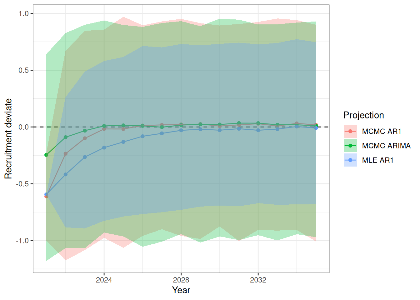
Summaries ARIMA pars, never any I which makes sense given ADF test..
melt(proj_rdev_ARIMA$arima_pars) %>%
  ggplot(aes(x = factor(statistic), y = value)) +
  geom_boxplot() +
  labs(x = "Statistic", y = "Order")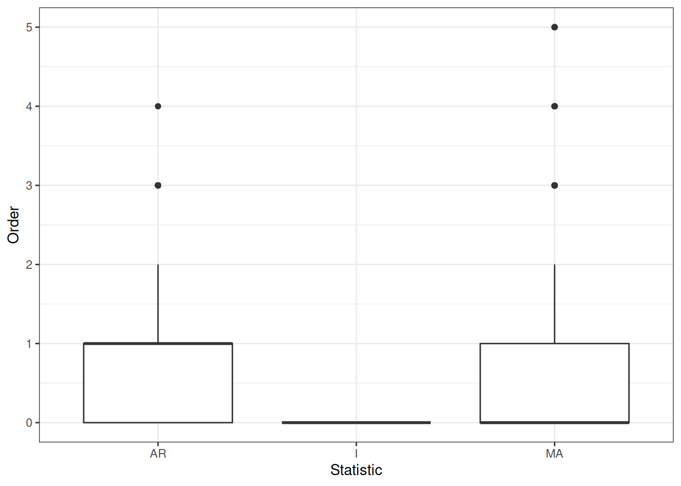
Selectivity
Projecting selectivity can be done using the project_selectivity function. The first_yr and the last_yr arguments define the range of years over which the mean and standard deviation of selectivity is calculated. Future selectivity is then drawn from a normal distribution (in log-space). Ridge plots of projected selectivity for a single iteration and the median are shown in Figure 10 and Figure 11. A line plot of median projected selectivity is shown in Figure 12.
# proj_sel_fya <- project_selectivity(
#   data = data, obj = obj, mcmc = mcmc, first_yr = 2021, last_yr = 2035,
#   samp_years = 2015:2020, iters = iters
# )
# save(proj_sel_fya, file = "inst/extdata/proj_sel.rda")
load(system.file("extdata", "proj_sel.rda", package = "sbt"))
# plot_selectivity(data = data, object = obj, years = 2015:2022, fisheries = "LL3")

library(ggridges)
library(scales)

fsh <- c("LL1", "LL2", "LL3", "LL4", "Indonesian", "Australian", "CPUE")

df <- melt(proj_sel_fya) %>%
  mutate(fishery = fsh[fishery]) %>%
  mutate(fishery = factor(fishery, levels = fsh)) %>%
  filter(iteration == 10)

ggplot(data = df, aes(x = age, y = year, height = value, group = year)) +
  geom_density_ridges(stat = "identity", alpha = 0.5, rel_min_height = 0) +
  facet_wrap(fishery ~ .) +
  labs(x = "Age", y = "Year") +
  theme(legend.position = "none") +
  scale_x_continuous(limits = c(0, NA), expand = expansion(mult = c(0, 0.05))) +
  scale_y_reverse(breaks = pretty_breaks())
Warning in FUN(X[[i]], ...): no non-missing arguments to max; returning -Inf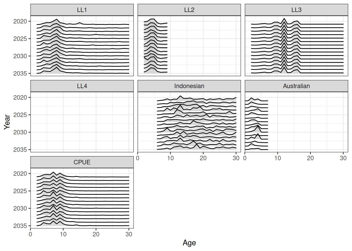
df <- melt(proj_sel_fya) %>%
  mutate(fishery = fsh[fishery]) %>%
  mutate(fishery = factor(fishery, levels = fsh)) %>%
  group_by(fishery, year, age) %>%
  summarise(value = median(value))

ggplot(data = df, aes(x = age, y = year, height = value, group = year)) +
  geom_density_ridges(stat = "identity", alpha = 0.5, rel_min_height = 0) +
  facet_wrap(fishery ~ .) +
  labs(x = "Age", y = "Year") +
  theme(legend.position = "none") +
  scale_x_continuous(limits = c(0, NA), expand = expansion(mult = c(0, 0.05))) +
  scale_y_reverse(breaks = pretty_breaks())
Warning in FUN(X[[i]], ...): no non-missing arguments to max; returning -Inf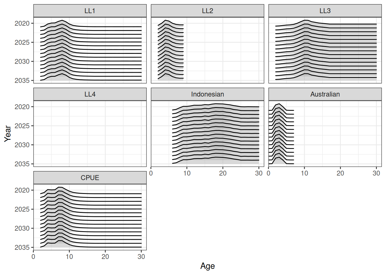
ggplot(data = df) +
  geom_line(aes(x = age, y = value, color = factor(year), group = year)) +
  facet_wrap(fishery ~ .) +
  scale_y_continuous(limits = c(0, NA), expand = expansion(mult = c(0, 0.05))) +
  labs(x = "Age", y = "Selectivity", color = "Year")
Warning: Removed 1335 rows containing missing values or values outside the scale range
(`geom_line()`).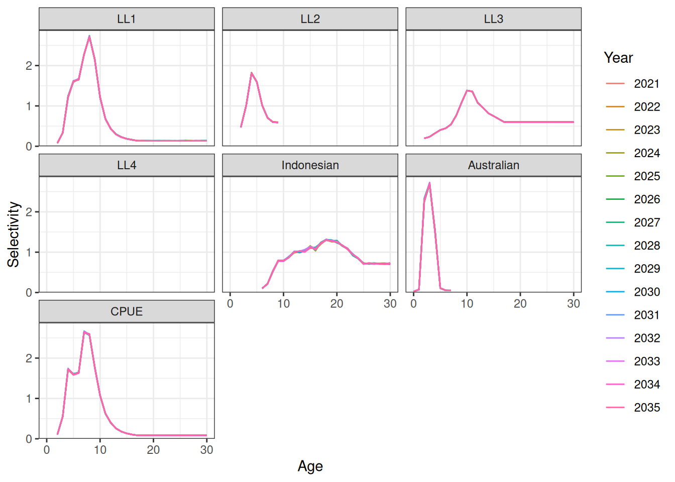
Catch
Projected catch by fishery is shown in Figure 13.
plot_catch(data = data, object = obj, proj = proj_catch_ysf)[1] "The maximum catch difference was: NA"Warning: Removed 65 rows containing missing values or values outside the scale range
(`geom_line()`).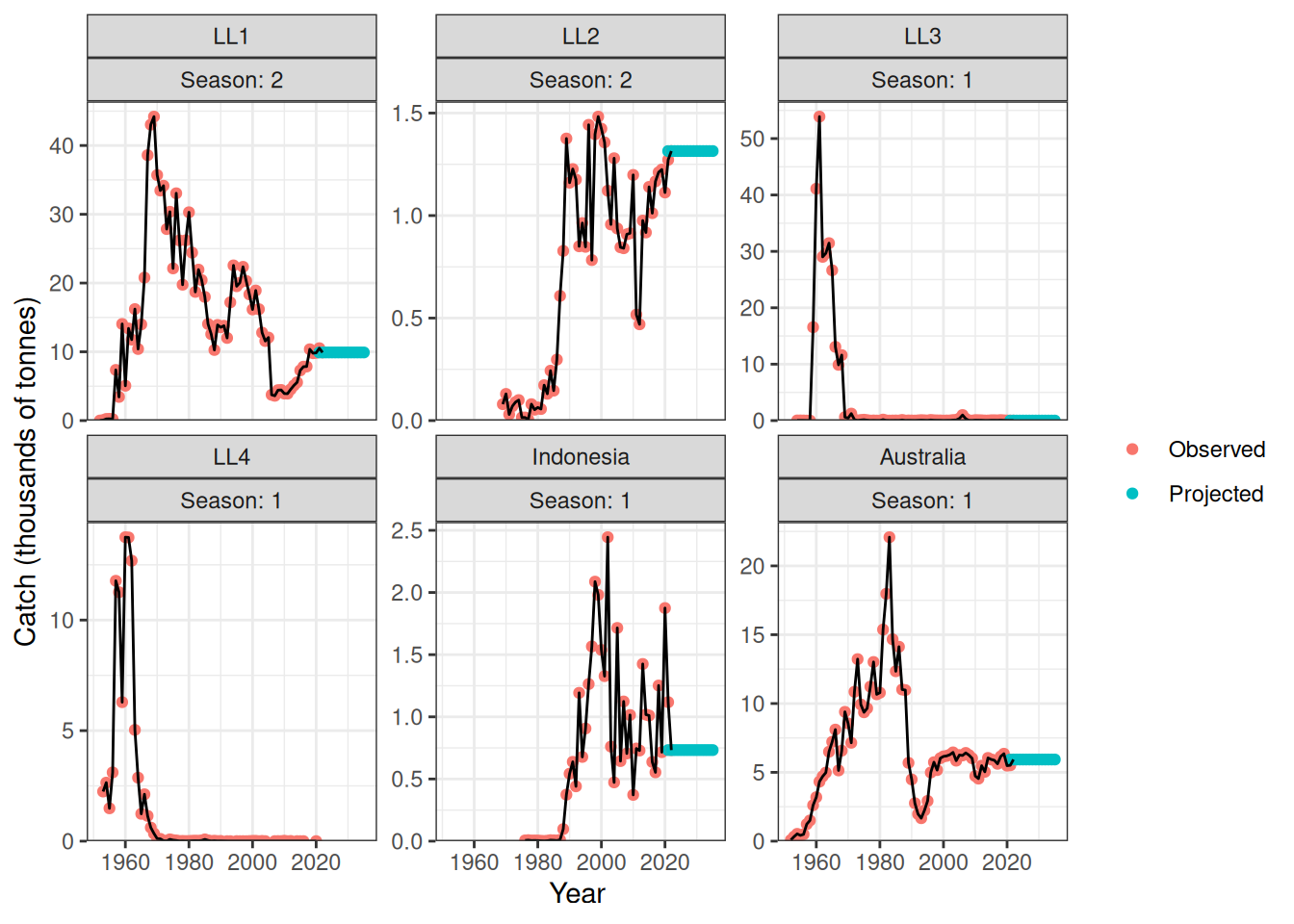
Projection using dynamics function
Project forward with MCMC different because not the MLE like everything else above (single MCMC iteration).
# proj_dyn <- project_dynamics(data = data, object = obj, mcmc = mcmc,
#                          first_yr = 2021, last_yr = 2035, n_iter = n_iter,
#                          rdev_y = proj_rdev_ARIMA$proj_rdev_y, sel_fya = proj_sel_fya,
#                          catch_ysf = proj_catch_ysf)
# save(proj_dyn, file = "inst/extdata/proj_dyn.rda")
load(system.file("extdata", "proj_dyn.rda", package = "sbt"))

df2 <- data.frame(year = (data$last_yr + 1):(data$last_yr + n_proj + 1),
                  value = proj_dyn[[1]]$spawning_biomass_y)

dim(proj_dyn[[1]]$number_ysa)
[1] 16 2 31
dimnames(proj_dyn[[1]]$number_ysa) <- list(year = 1:16, season = 1:2, age = data$age_a)

# post <- extract_samples(fit = mcmc)
# plot(data$first_yr:(data$last_yr + 1), obj$report()$spawning_biomass_y, xlim = c(1931, max(proj_years)), ylim = c(0, 11e6))
# # for (i in seq_len(n_iter)) {
# for (i in seq_len(10)) {
#   rep <- obj$report(as.numeric(post[i,]))
#   lines(data$first_yr:(data$last_yr + 1), rep$spawning_biomass_y, col = 3)
#   lines(min(proj_years):(max(proj_years) + 1), dyn4[[i]]$spawning_biomass_y, col = 4)
# }
#
# plot(data$cpue_years + data$first_yr - 1, data$cpue_obs, xlim = c(1969, 2042), ylim = c(0.3, 4))
# # for (i in seq_len(n_iter)) {
# for (i in seq_len(10)) {
#   rep <- obj$report(as.numeric(post[i,]))
#   lines(data$cpue_years + data$first_yr - 1, rep$cpue_pred, col = 2)
#   lines(proj_years, dyn4[[i]]$cpue_pred, col = 3)
#   points(proj_years, dyn4[[i]]$cpue_obs, col = 4)
# }