Introduction
The sbt software is an R package (R Core Team 2024) that contains the CCSBT operating model (OM) coded using RTMB Kristensen (2025). This page provides examples using the sbt model.
Load inputs
If you have not done so already, you will need to install the packages below:
The sbt RTMB model is loaded along with several R functions using library(sbt). The tidyverse and reshape2 packages are used for data manipulation and plotting. The code theme_set(theme_bw()) alters the plot aesthetics of the entire article
The data list is defined below and then the get_data function is used to set up some additional inputs that are required before the data list can be passed to MakeADFun.
data <- list(
  last_yr = 2022, age_increase_M = 25, length_m50 = 150, length_m95 = 180,
  catch_UR_on = 0, catch_surf_case = 1, catch_LL1_case = 1,
  scenarios_surf = data_csv1$scenarios_surface,
  scenarios_LL1 = data_csv1$scenarios_LL1,
  removal_switch_f = c(0, 0, 0, 1, 0, 0), # 0=harvest rate, 1=direct removals
  sel_min_age_f = c(2, 2, 2, 8, 6, 0, 2),
  sel_max_age_f = c(17, 9, 17, 22, 25, 7, 17),
  sel_end_f = c(1, 0, 1, 1, 1, 0, 1),
  sel_LL1_yrs = c(1952, 1957, 1961, 1965, 1969, 1973, 1977, 1981, 1985, 1989,
                  1993, 1997, 2001, 2006, 2007, 2008, 2011, 2014, 2017, 2020),
  sel_LL2_yrs = c(1969, 2001, 2005, 2008, 2011, 2014, 2017, 2020),
  sel_LL3_yrs = c(1954, 1961, 1965, 1969, 1970, 1971, 2005, 2006, 2007),
  sel_LL4_yrs = c(1953),
  sel_Ind_yrs = c(1976, 1995, 1997, 1999, 2002, 2004, 2006, 2008, 2010, 2012,
                  2013, 2014, 2015, 2016, 2017, 2018, 2019, 2020, 2021, 2022),
  sel_Aus_yrs = c(1952, 1969, 1973, 1977, 1981, 1985, 1989, 1993, 1997, 1998,
                  1999, 2000, 2001, 2002, 2003, 2004, 2005, 2006, 2007, 2008,
                  2009, 2010, 2011, 2012, 2013, 2014, 2015, 2016, 2017, 2018,
                  2019, 2020, 2021, 2022),
  sel_CPUE_yrs = c(1969, 1973, 1977, 1981, 1985, 1989, 1993, 1997, 2001, 2006,
                   2007, 2008, 2011, 2014, 2017, 2020),
  af_switch = 9,
  lf_switch = 9, lf_minbin = c(1, 1, 1, 11),
  cpue_switch = 1, cpue_a1 = 5, cpue_a2 = 17,
  troll_switch = 1,
  aerial_switch = 4, aerial_tau = 0.3,
  tag_switch = 1, tag_var_factor = 1.82,
  hsp_switch = 1, hsp_false_negative = 0.7467647,
  pop_switch = 1,
  gt_switch = 1
)

data <- get_data(data_in = data)
names(data) [1] "last_yr" "age_increase_M" "length_m50"
[4] "length_m95" "removal_switch_f" "sel_min_age_f"
[7] "sel_max_age_f" "sel_end_f" "af_switch"
[10] "lf_switch" "lf_minbin" "cpue_switch"
[13] "cpue_a1" "cpue_a2" "troll_switch"
[16] "aerial_switch" "aerial_tau" "tag_switch"
[19] "tag_var_factor" "hsp_switch" "hsp_false_negative"
[22] "pop_switch" "gt_switch" "first_yr"
[25] "n_year" "n_season" "min_age"
[28] "max_age" "n_age" "n_length"
[31] "n_fishery" "age_a" "length_mu_ysa"
[34] "length_sd_a" "weight_fya" "first_yr_catch"
[37] "first_yr_catch_f" "n_catch" "catch_year"
[40] "catch_obs_ysf" "sel_change_year_fy" "pop_obs"
[43] "paly" "hsp_obs" "gt_obs"
[46] "aerial_survey" "troll_years" "troll_obs"
[49] "troll_sd" "cpue_years" "cpue_obs"
[52] "cpue_sd" "af_min_age" "af_max_age"
[55] "n_af" "af_year" "af_fishery"
[58] "af_obs" "af_n" "dl_yal"
[61] "alk_ysal" "lf_year" "lf_fishery"
[64] "lf_season" "lf_obs" "lf_n"
[67] "lf_slices" "af_sliced" "af_sliced_ysfa"
[70] "cpue_lfs" "cpue_n" "tag_shed_immediate"
[73] "tag_shed_continuous" "tag_rep_rates_ya" "tag_rel_min_age"
[76] "tag_rel_max_age" "tag_release_cta" "tag_recap_ctaa"
[79] "tag_recap_max_age" "min_K" "n_K"
[82] "n_T" "n_I" "n_J" Input tables
The fleets (Table 1).
| Fishery fleet | Primary Nations / Components | Gear type | Key characteristics in assessment |
|---|---|---|---|
| LL1 | Japan | Longline | Provides the primary standardised CPUE index for adult abundance. |
| LL2 | Korea & Taiwan | Longline | Combined data for Northeast Asian longline fleets; distinct selectivity. |
| LL3 | Other Longline | Longline | Catch from smaller fleets and non-member effort not in LL1, LL2, or LL4. |
| LL4 | New Zealand | Longline | Specifically the NZ domestic and charter longline fishery data. |
| Indonesian | Indonesia | Longline | Operates on spawning grounds (Area 1); catches oldest mature fish. |
| Australian surface | Australia | Purse Seine | Targets juveniles (ages 2–4) in the GAB for ranching/farming. |
| Fishery | Description | Season |
|---|---|---|
| LL1 | Japanese LL areas 4-9 and other longline catches | 2 |
| LL2 | Taiwanese albacore LL and gillnet | 2 |
| LL3 | Japanese LL in Area 2 | 1 |
| LL4 | Japanese spawning (Area 1) | 1 |
| Indonesian | Indonesian spawning | 1 |
| Australian Surface | Surface fishery | 1 |
| CPUE block | Selectivity-only block used in the CPUE likelihood | 2 |
Below are examples of some of the model inputs in tabular form. Mean lengths by year, season, and age are shown in Table 2. The parent offspring pair data are shown in Table 3. The unaccounted catch data are shown in Table 6.
| Year | Season | 0 | 1 | 2 | 3 | 4 | 5 | 6 | 7 | 8 | 9 | 10 |
|---|---|---|---|---|---|---|---|---|---|---|---|---|
| 1931 | 1 | 45 | 57.1 | 74.1 | 88.8 | 101.8 | 113.9 | 124.3 | 133.3 | 141.0 | 147.6 | 153.3 |
| 1932 | 1 | 45 | 57.1 | 74.1 | 88.8 | 101.8 | 113.9 | 124.3 | 133.3 | 141.0 | 147.6 | 153.3 |
| 1933 | 1 | 45 | 57.1 | 74.1 | 88.8 | 101.8 | 113.9 | 124.3 | 133.3 | 141.0 | 147.6 | 153.3 |
| 1934 | 1 | 45 | 57.1 | 74.1 | 88.8 | 101.8 | 113.9 | 124.3 | 133.3 | 141.0 | 147.6 | 153.3 |
| 1935 | 1 | 45 | 57.1 | 74.1 | 88.8 | 101.8 | 113.9 | 124.3 | 133.3 | 141.0 | 147.6 | 153.3 |
| 1936 | 1 | 45 | 57.1 | 74.1 | 88.8 | 101.8 | 113.9 | 124.3 | 133.3 | 141.0 | 147.6 | 153.3 |
| 2017 | 2 | 50 | 68.9 | 91.6 | 105.5 | 117.3 | 127.2 | 135.6 | 142.7 | 148.7 | 153.8 | 158.1 |
| 2018 | 2 | 50 | 68.9 | 91.6 | 105.5 | 117.3 | 127.2 | 135.6 | 142.7 | 148.7 | 153.8 | 158.1 |
| 2019 | 2 | 50 | 68.9 | 91.6 | 105.5 | 117.3 | 127.2 | 135.6 | 142.7 | 148.7 | 153.8 | 158.1 |
| 2020 | 2 | 50 | 68.9 | 91.6 | 105.5 | 117.3 | 127.2 | 135.6 | 142.7 | 148.7 | 153.8 | 158.1 |
| 2021 | 2 | 50 | 68.9 | 91.6 | 105.5 | 117.3 | 127.2 | 135.6 | 142.7 | 148.7 | 153.8 | 158.1 |
| 2022 | 2 | 50 | 68.9 | 91.6 | 105.5 | 117.3 | 127.2 | 135.6 | 142.7 | 148.7 | 153.8 | 158.1 |
| Cohort | CaptureYear | CaptureCov | CaptureSwitch | NPOPS | Comps |
|---|---|---|---|---|---|
| 2007 | 2012 | 15 | 1 | 0 | 1315 |
| 2008 | 2012 | 15 | 1 | 0 | 963 |
| 2009 | 2012 | 15 | 1 | 0 | 876 |
| 2010 | 2012 | 15 | 1 | 0 | 903 |
| 2011 | 2012 | 15 | 1 | 0 | 899 |
| 2003 | 2013 | 15 | 1 | 0 | 1317 |
| 2004 | 2013 | 15 | 1 | 0 | 1325 |
| 2005 | 2013 | 15 | 1 | 0 | 1356 |
| 2006 | 2013 | 15 | 1 | 0 | 1347 |
| 2007 | 2013 | 15 | 1 | 0 | 1315 |
| 2008 | 2013 | 15 | 1 | 0 | 963 |
| 2009 | 2013 | 15 | 1 | 0 | 876 |
| 2010 | 2013 | 15 | 1 | 0 | 903 |
| 2011 | 2013 | 15 | 1 | 0 | 899 |
| 2012 | 2013 | 15 | 1 | 0 | 953 |
| cohort1 | cohort2 | nC | nK |
|---|---|---|---|
| 2013 | 2014 | 809592 | 4 |
| 2013 | 2015 | 645624 | 1 |
| 2013 | 2016 | 1237446 | 0 |
| 2013 | 2017 | 1291248 | 1 |
| 2013 | 2018 | 1181936 | 0 |
| 2014 | 2015 | 716688 | 2 |
| 2014 | 2016 | 1373652 | 1 |
| 2014 | 2017 | 1433376 | 4 |
| 2014 | 2018 | 1312032 | 3 |
| 2015 | 2016 | 1095444 | 2 |
| 2015 | 2017 | 1143072 | 1 |
| 2015 | 2018 | 1046304 | 3 |
| 2016 | 2017 | 2190888 | 4 |
| 2016 | 2018 | 2005416 | 5 |
| 2017 | 2018 | 2092608 | 2 |
| Release year | Release age | Recapture year | Number released | Number sampled | Number of matches |
|---|---|---|---|---|---|
| 2016 | 2 | 2017 | 2952 | 15389 | 20 |
| 2017 | 2 | 2018 | 6480 | 11932 | 67 |
| 2018 | 2 | 2019 | 6295 | 11980 | 66 |
| 2019 | 2 | 2020 | 4242 | 11109 | 31 |
| 2021 | 2 | 2022 | 6401 | 10742 | 41 |
| Year | LL1 | LL2 | LL3 | LL4 | Indonesia | Australia |
|---|---|---|---|---|---|---|
| 2008 | 72 | 0 | 0 | 0 | 0 | 0 |
| 2009 | 152 | 0 | 0 | 0 | 0 | 0 |
| 2010 | 271 | 0 | 0 | 0 | 0 | 0 |
| 2011 | 151 | 0 | 0 | 0 | 0 | 0 |
| 2012 | 275 | 0 | 0 | 0 | 0 | 0 |
| 2013 | 432 | 0 | 0 | 0 | 0 | 0 |
| 2014 | 121 | 0 | 0 | 0 | 0 | 0 |
| 2015 | 326 | 0 | 0 | 0 | 0 | 0 |
| 2016 | 756 | 0 | 0 | 0 | 0 | 0 |
| 2017 | 984 | 0 | 0 | 0 | 0 | 0 |
| 2018 | 1511 | 0 | 0 | 0 | 0 | 0 |
| 2019 | 1155 | 0 | 0 | 0 | 0 | 0 |
| 2020 | 1160 | 0 | 0 | 0 | 0 | 0 |
| 2021 | 1160 | 0 | 0 | 0 | 0 | 0 |
| 2022 | 1160 | 0 | 0 | 0 | 0 | 0 |
Input plots
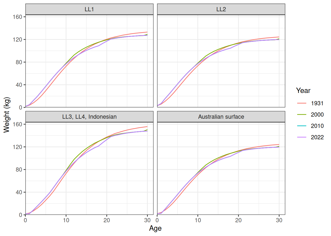
Length at age (Figure 1). Weight at age (Figure 2).
plot_length_at_age(data = data, years = c(1931, 2022))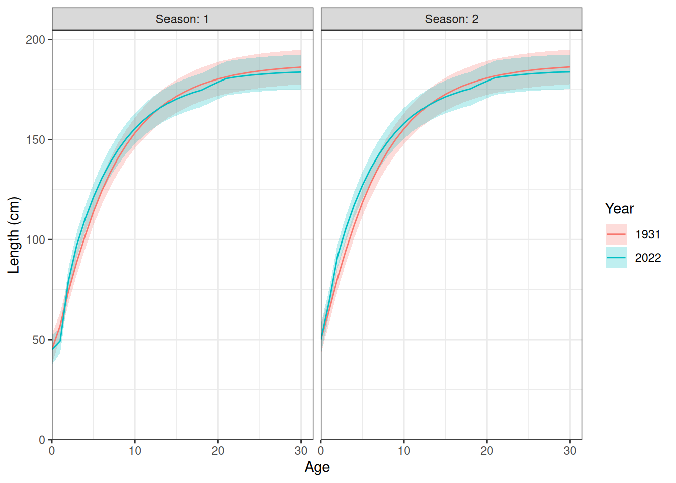
plot_weight_at_age(data = data, years = c(1931, 2000, 2010, 2022))