Introduction
Bayesian inference for a TMB model can be done using
tmbstan which makes use of Stan’s Markov chain Monte Carlo
(MCMC) algorithm, specifically the no U-turn sampler (NUTS). In this
vignette, a model run is setup, frequentist optimisation is done, and
then MCMC is used to obtain samples from the posterior distribution.
Model setup
Below the required R libraries are loaded:
library(tidyverse)
library(sbt)
library(tmbstan)
library(kableExtra)
library(bayesplot)

theme_set(theme_bw())

# Specify the number of cores for MCMC
options(mc.cores = parallel::detectCores())
Example inputs are loaded from the sbt package:
attach(data_csv1)Normally the user would import these inputs (e.g., from
.csv files using the read_csv function).
The input data list is defined and then the get_data
function is used to set up some additional inputs that are required
before the data list can be passed to MakeADFun:
Data <- list(last_yr = 2022, age_increase_M = 25,
             length_m50 = 150, length_m95 = 180,
             catch_UR_on = 0, catch_surf_case = 1, catch_LL1_case = 1,
             scenarios_surf = scenarios_surface, scenarios_LL1 = scenarios_LL1,
             sel_min_age_f = c(2, 2, 2, 8, 6, 0),
             sel_max_age_f = c(17, 9, 17, 22, 25, 7),
             sel_end_f = c(1, 0, 1, 1, 1, 0),
             sel_change_sd_fy = t(as.matrix(sel_change_sd[,-1])),
             sel_smooth_sd_f = data_labrep1$sel.smooth.sd,
             removal_switch = c(0, 0, 0, 0, 0, 0), # 0=standard, 1=direct
             pop_switch = 1,
             hsp_switch = 1, hsp_false_negative = 0.7467647,
             gt_switch = 1,
             cpue_switch = 1, cpue_a1 = 5, cpue_a2 = 17,
             aerial_switch = 4, aerial_tau = data_labrep1$tau.aerial,
             troll_switch = 0,
             af_switch = 3,
             lf_switch = 3, lf_minbin = c(1, 1, 1, 11),
             tag_switch = 1, tag_var_factor = 1.82
)

Data <- get_data(data_in = Data)
The parameter list is defined:
Params <- list(par_log_B0 = data_par1$ln_B0,
               par_log_psi = log(data_par1$psi),
               par_log_m0 = log(data_par1$m0),
               par_log_m4 = log(data_par1$m4),
               par_log_m10 = log(data_par1$m10),
               par_log_m30 = log(data_par1$m30),
               par_log_h = log(data_par1$steep),
               par_log_sigma_r = log(data_labrep1$sigma.r),
               par_log_cpue_q = data_par1$lnq,
               par_log_cpue_sigma = log(data_par1$sigma_cpue),
               par_log_cpue_omega = log(data_par1$cpue_omega),
               par_log_aerial_tau = log(data_par1$tau_aerial),
               par_log_aerial_sel = data_par1$ln_sel_aerial,
               par_log_troll_tau = log(data_par1$tau_troll),
               par_log_hsp_q = data_par1$lnqhsp,
               par_log_tag_H_factor = log(data_par1$tag_H_factor),
               par_log_af_alpha = c(1, 1),
               par_log_lf_alpha = c(1, 1, 1, 1),
               par_rdev_y = data_par1$Reps,
               par_sels_init_i = data_par1$par_sels_init_i,
               par_sels_change_i = data_par1$par_sels_change_i
)
TMB’s map option can be used to turn parameters
on/off:
Map <- list()
Map[["par_log_psi"]] <- factor(NA)
Map[["par_log_h"]] <- factor(NA)
Map[["par_log_sigma_r"]] <- factor(NA)
Map[["par_log_cpue_sigma"]] <- factor(NA)
Map[["par_log_cpue_omega"]] <- factor(NA)
Map[["par_log_aerial_tau"]] <- factor(NA)
Map[["par_log_aerial_sel"]] <- factor(rep(NA, 2))
Map[["par_log_troll_tau"]] <- factor(NA)
Map[["par_log_hsp_q"]] <- factor(NA)
Map[["par_log_tag_H_factor"]] <- factor(NA)
Map[["par_log_af_alpha"]] <- factor(rep(NA, 2))
Map[["par_log_lf_alpha"]] <- factor(rep(NA, 4))
Finally, the AD object is created using TMBs MakeADFun
function:
obj <- MakeADFun(data = Data, parameters = Params, map = Map, random = c(),
                 hessian = TRUE, inner.control = list(maxit = 50), DLL = "sbt")
#> Constructing atomic D_lgamma
A list of the parameters that are to be estimated can be generated using:
unique(names(obj$par))
#> [1] "par_log_B0"        "par_log_m0"        "par_log_m4"
#> [4] "par_log_m10"       "par_log_m30"       "par_log_cpue_q"
#> [7] "par_rdev_y"        "par_sels_init_i"   "par_sels_change_i"
And the objective function value given the initial values is:
obj$fn(obj$par)
#> [1] 27328.36
Optimisation
Load the default parameter bounds:
bnd <- get_bounds(obj = obj)
head(bnd)
#>        parameter        init     lower      upper
#> 1     par_log_B0 16.19836436      -Inf        Inf
#> 2     par_log_m0 -0.91629073 -1.609438 -0.5978370
#> 3     par_log_m4 -1.78945804 -2.733368 -1.2432509
#> 4    par_log_m10 -2.73336801 -3.540459 -1.5606477
#> 5    par_log_m30 -0.78217510 -1.609438 -0.3566749
#> 6 par_log_cpue_q -0.02033773      -Inf        Inf
Optimise using the nlminb function:
control <- list(eval.max = 200000, iter.max = 200000)

opt <- nlminb(start = obj$par, objective = obj$fn, gradient = obj$gr,
              lower = bnd$lower, upper = bnd$upper, control = control)
#> Warning in nlminb(start = obj$par, objective = obj$fn, gradient = obj$gr, :
#> NA/NaN function evaluation
#> Warning in nlminb(start = obj$par, objective = obj$fn, gradient = obj$gr, :
#> NA/NaN function evaluation
# opt <- optim(par = obj$par, fn = obj$fn, gr = obj$gr, method = "L-BFGS-B",
#              lower = bnd$lower, upper = bnd$upper)
Markov chain Monte Carlo
Samples from the posterior distribution are obtained using
tmbstan and output to a stanfit object, in
this case called mcmc1:
if (FALSE) {
  mcmc1 <- tmbstan(obj = obj, init = rep(list(Params), 2),
                   lower = bnd$lower, upper = bnd$upper, chains = 2,
                   control = list(max_treedepth = 12, adapt_delta = 0.9))
  save(mcmc1, file = "mcmc1.rda")
} else {
  load("mcmc1.rda")
}

get_elapsed_time(object = mcmc1) / 60 / 60 # elapsed time in hours
#>           warmup   sample
#> chain:1 5.301972 5.422861
#> chain:2 5.379639 3.845639
MCMC diagnostics
Several MCMC diagnostics outputs are presented below. In this example, several iterations ended with a divergence. There should be no divergent transitions if samples from the posterior distribution are to be used for inference.
check_hmc_diagnostics(object = mcmc1)
#>
#> Divergences:
#> 94 of 2000 iterations ended with a divergence (4.7%).
#> Try increasing 'adapt_delta' to remove the divergences.
#>
#> Tree depth:
#> 0 of 2000 iterations saturated the maximum tree depth of 12.
#>
#> Energy:
#> E-BFMI indicated no pathological behavior.
In the MCMC summary table below, the effective number of samples
should be greater than 400 and the Rhat statistic should be
less than 1.01 for all model parameters:
pars <- c("lp__", "par_log_B0", "par_log_m0", "par_log_m4", "par_log_m10",
          "par_log_m30", "par_log_cpue_q",
          "par_rdev_y[1]", "par_rdev_y[92]",
          "par_sels_init_i[1]", "par_sels_init_i[78]",
          "par_sels_change_i[1]", "par_sels_change_i[1132]")

df <- summary(mcmc1, pars = pars)$summary %>%
  data.frame() %>%
  mutate(Parameter = row.names(.)) %>%
  select(Parameter, mean, X2.5., X50., X97.5., n_eff, Rhat)
row.names(df) <- NULL
cnames <- c("Parameter", "Mean", "2.5%", "Median", "97.5%", "Eff. N", "Rhat")

kbl(x = df, digits = 3, col.names = cnames) %>%
  kable_styling("bordered") %>%
  kable_styling() %>%
  column_spec(column = 6, color = ifelse(df$n_eff <= 400, "red", "black")) %>%
column_spec(column = 7, color = ifelse(df$Rhat >= 1.01, "red", "black"))| Parameter | Mean | 2.5% | Median | 97.5% | Eff. N | Rhat |
|---|---|---|---|---|---|---|
| lp__ | -27699.140 | -27751.830 | -27697.821 | -27650.521 | 640.302 | 1.002 |
| par_log_B0 | 15.888 | 15.576 | 15.886 | 16.221 | 567.976 | 1.002 |
| par_log_m0 | -0.836 | -1.019 | -0.830 | -0.669 | 1855.946 | 1.000 |
| par_log_m4 | -1.854 | -1.981 | -1.852 | -1.730 | 1268.803 | 0.999 |
| par_log_m10 | -2.315 | -2.673 | -2.295 | -2.039 | 602.812 | 1.000 |
| par_log_m30 | -0.854 | -1.075 | -0.852 | -0.639 | 1887.222 | 1.001 |
| par_log_cpue_q | -0.017 | -0.073 | -0.016 | 0.042 | 2602.108 | 0.999 |
| par_rdev_y[1] | -0.014 | -1.230 | -0.016 | 1.193 | 2690.793 | 1.000 |
| par_rdev_y[92] | -0.007 | -1.066 | -0.004 | 1.005 | 2688.725 | 1.001 |
| par_sels_init_i[1] | -4.939 | -7.726 | -4.853 | -2.723 | 1100.721 | 0.999 |
| par_sels_init_i[78] | 1.135 | 0.874 | 1.133 | 1.377 | 2335.212 | 1.000 |
| par_sels_change_i[1] | 0.790 | -1.532 | 0.731 | 3.342 | 1454.511 | 0.999 |
| par_sels_change_i[1132] | 0.008 | -3.659 | 0.008 | 3.713 | 2885.593 | 1.000 |
rhats <- rhat(object = mcmc1)
rhats <- rhats[rhats > 1.004]
mcmc_rhat(rhat = rhats) + yaxis_text(hjust = 1)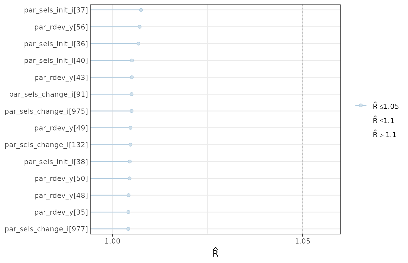
A subset of the worst model Rhats.
ratios <- neff_ratio(object = mcmc1)
ratios <- ratios[ratios < 0.25]
mcmc_neff(ratio = ratios) + yaxis_text(hjust = 1)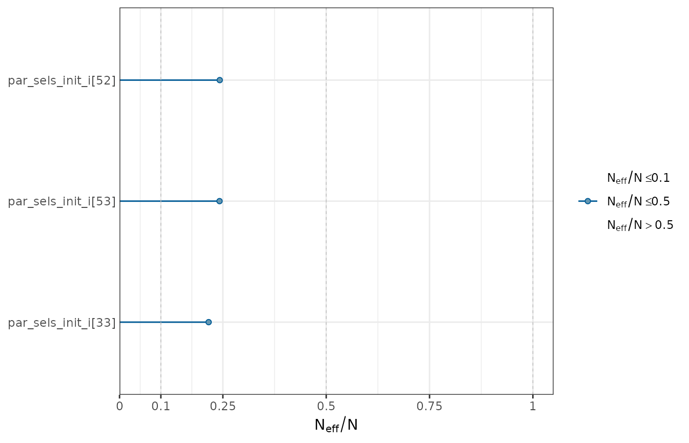
A subset of the worst ratios of effective sample size to total sample size.
nps <- nuts_params(object = mcmc1)
mcmc_trace(x = mcmc1, regex_pars = pars, np = nps, facet_args = list(ncol = 3))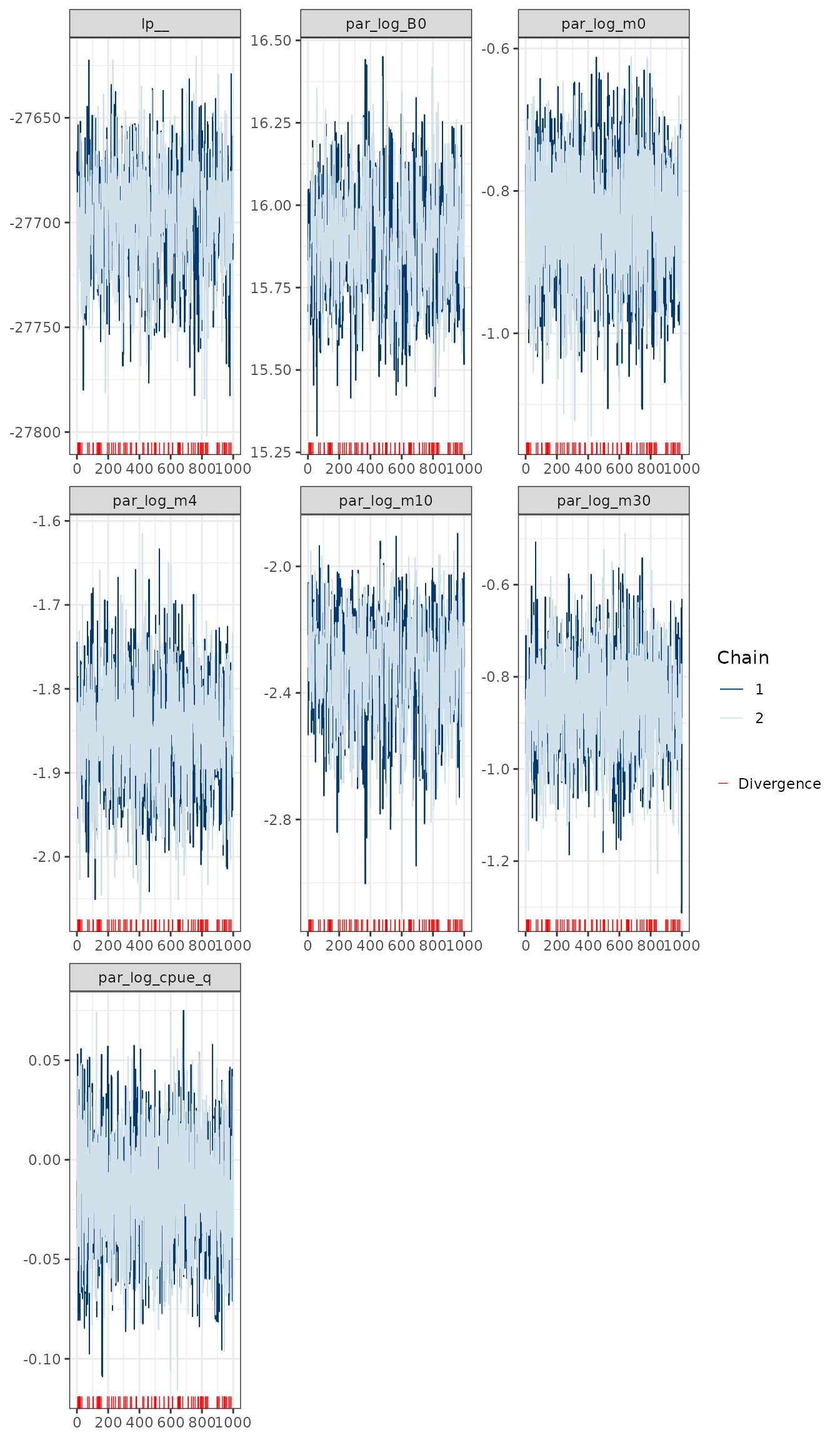
MCMC trace plots for some of the key model parameters.
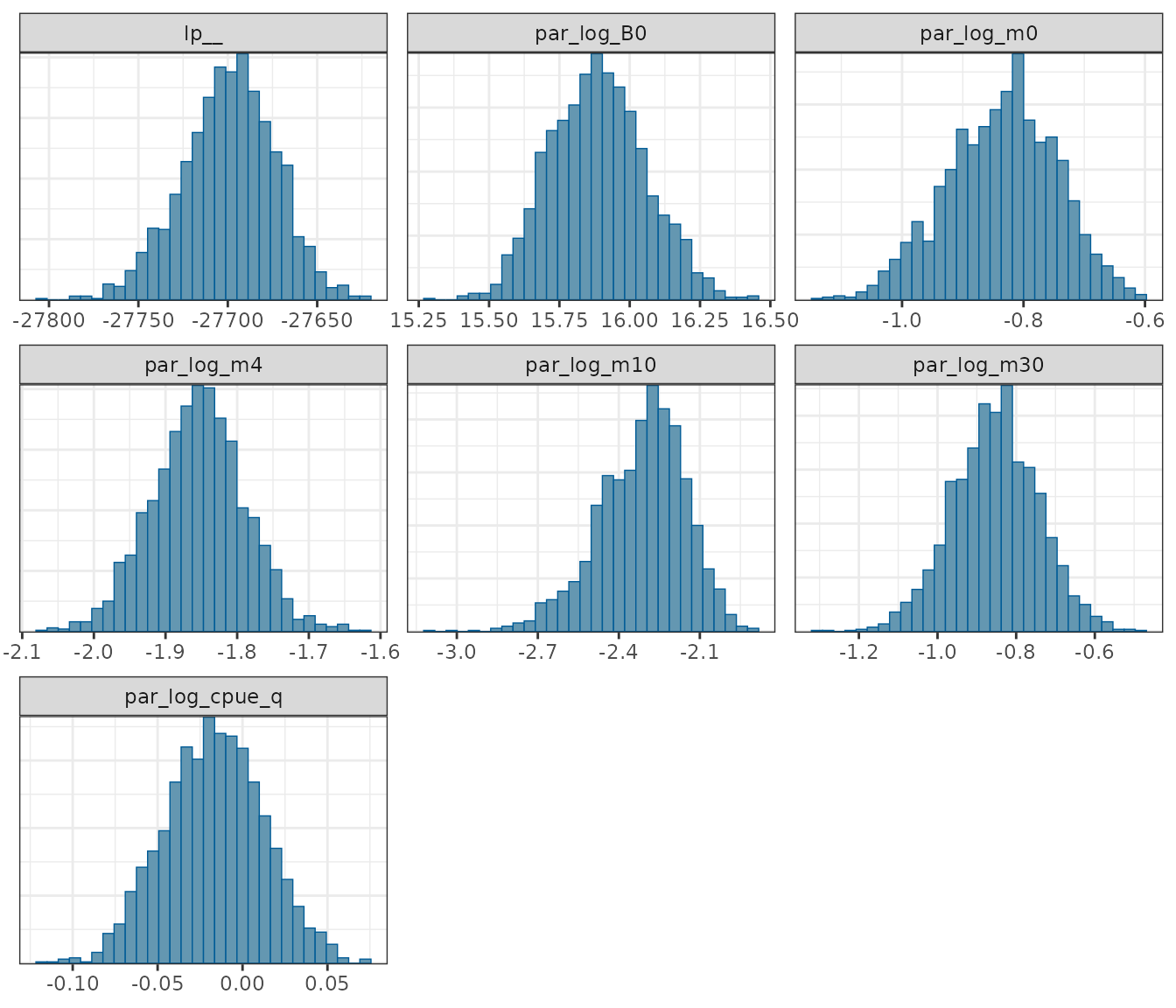
Posterior distribution histograms for some of the key model parameters.
Pairs plots can be used to help identify divergent transitions but are only useful for up to about 8 parameters:
pars <- c("par_log_B0", "par_log_m0", "par_log_m4", "par_log_m10",
          "par_log_m30", "par_log_cpue_q")
mcmc_pairs(x = mcmc1, pars = pars, np = nps)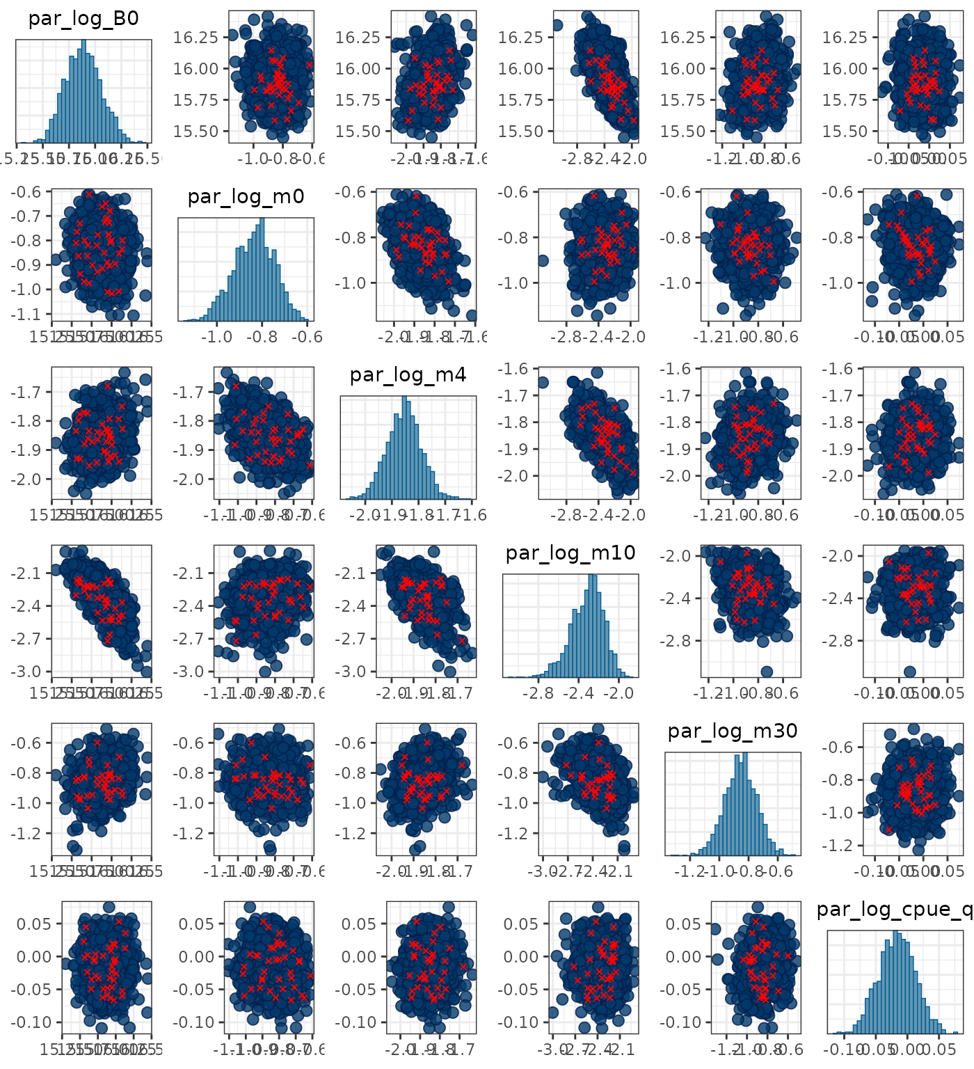
pars <- c("par_sels_init_i[33]", "par_sels_init_i[50]", "par_sels_init_i[51]",
          "par_sels_change_i[24]", "par_sels_change_i[25]")
mcmc_pairs(x = mcmc1, pars = pars, np = nps)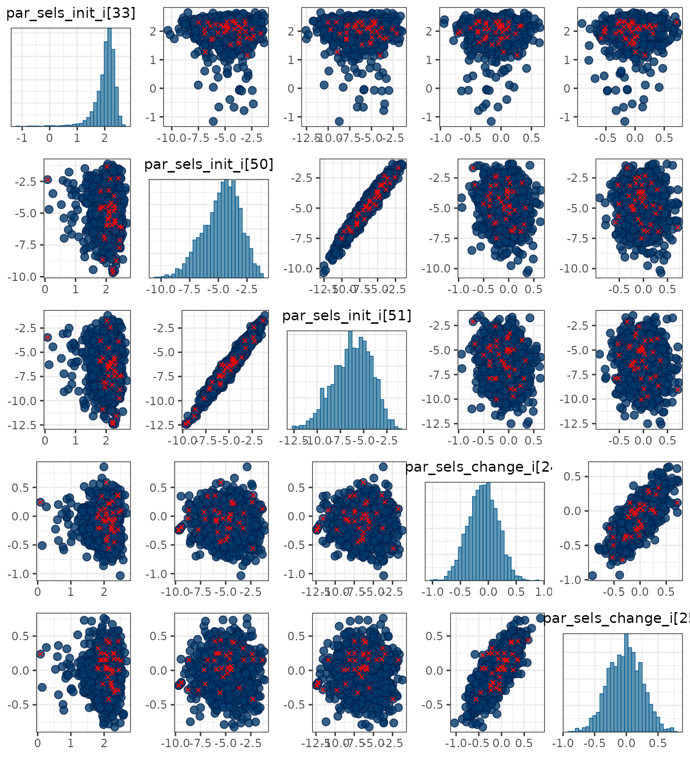
Parallel coordinates plots of MCMC draws have one dimension per parameter along the horizontal axis and each set of connected line segments represents a single MCMC draw (i.e., a vector of length equal to the number of parameters). Divergences are highlighted red in the plot. This version of the plot is the same as the parallel coordinates plot described in Gabry et al. (2019):
pars <- c("par_log_B0", "par_log_m0", "par_log_m4", "par_log_m10",
          "par_log_m30", "par_log_cpue_q", "par_rdev_y[1]", "par_rdev_y[92]")
mcmc_parcoord(mcmc1, pars = pars, np = nps,
              transform = function(x) {(x - mean(x)) / sd(x)}) +
  theme(axis.text.x = element_text(angle = 90, vjust = 0.5, hjust = 1))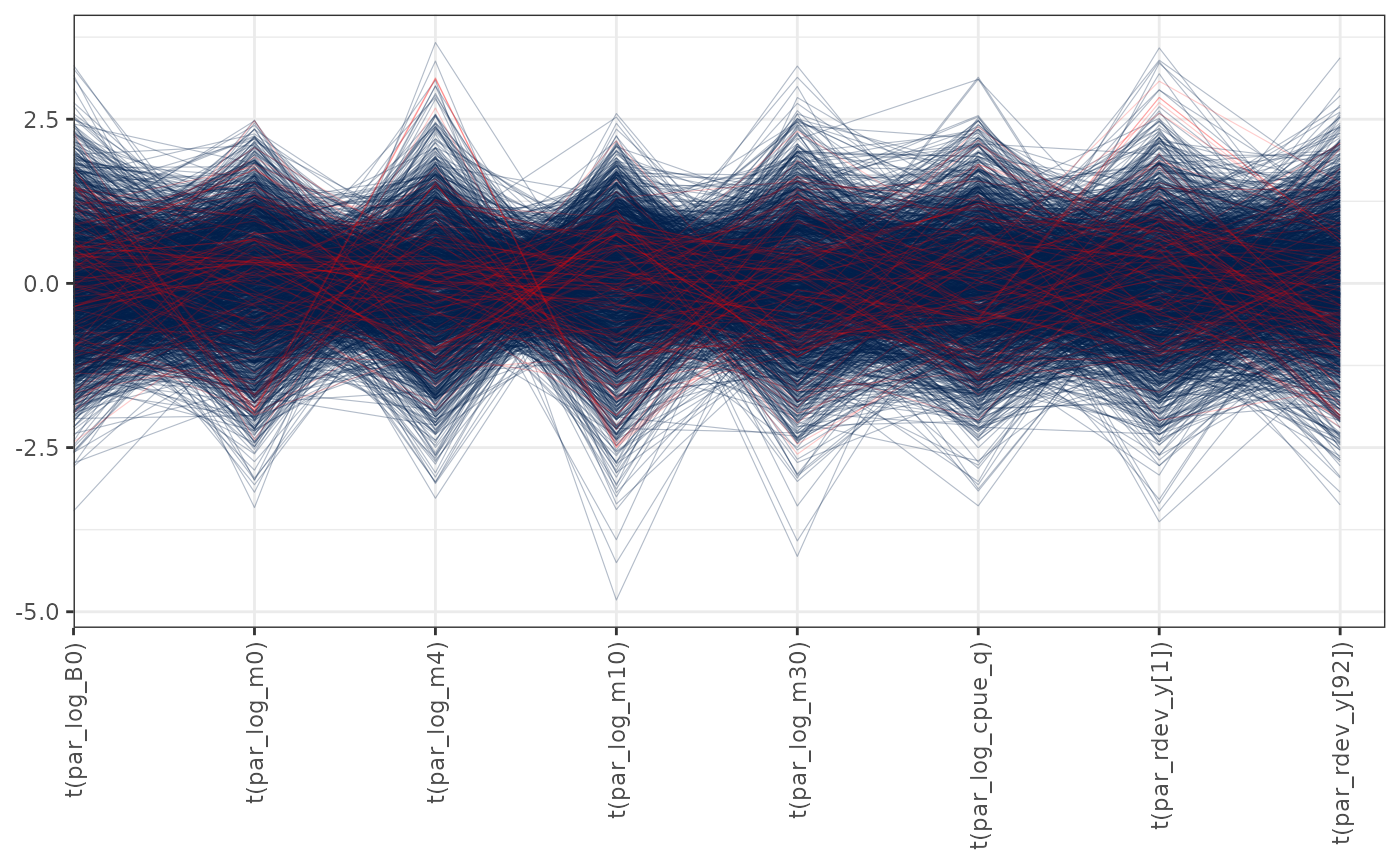
# mcmc_parcoord(x = mcmc1, regex_pars = "par_logit_hstar_i", np = nps) +
#   theme(axis.text.x = element_text(angle = 90, vjust = 0.5, hjust = 1))
get_sel_list(data = Data, opt = opt)
#> [[1]]
#>    id        par lower upper bound_check
#> 1   1 -4.5893007   -20   100          OK
#> 2   2 -3.9043100   -20   100          OK
#> 3   3 -3.1454645   -20   100          OK
#> 4   4 -2.3101183   -20   100          OK
#> 5   5 -1.3990471   -20   100          OK
#> 6   6 -0.4365832   -20   100          OK
#> 7   7  0.4923964   -20   100          OK
#> 8   8  1.2110336   -20   100          OK
#> 9   9  1.4924923   -20   100          OK
#> 10 10  1.2073934   -20   100          OK
#> 11 11  0.4086961   -20   100          OK
#> 12 12 -0.7386636   -20   100          OK
#> 13 13 -2.0719894   -20   100          OK
#> 14 14 -3.4827787   -20   100          OK
#> 15 15 -4.9194979   -20   100          OK
#> 16 16 -6.3678832   -20   100          OK
#>
#> [[2]]
#>   id        par lower upper bound_check
#> 1 17 -0.1490074   -20   100          OK
#> 2 18  0.7278095   -20   100          OK
#> 3 19  0.7332246   -20   100          OK
#> 4 20  0.2591719   -20   100          OK
#> 5 21 -0.3779382   -20   100          OK
#> 6 22 -0.9156792   -20   100          OK
#> 7 23 -1.2020650   -20   100          OK
#> 8 24 -1.1902027   -20   100          OK
#>
#> [[3]]
#>    id        par lower upper bound_check
#> 1  25 -7.9917990   -20   100          OK
#> 2  26 -6.5033369   -20   100          OK
#> 3  27 -5.8190469   -20   100          OK
#> 4  28 -5.8466844   -20   100          OK
#> 5  29 -5.5138385   -20   100          OK
#> 6  30 -3.0383934   -20   100          OK
#> 7  31  0.9531689   -20   100          OK
#> 8  32  1.2896868   -20   100          OK
#> 9  33  2.1643129   -20   100          OK
#> 10 34 -0.1428461   -20   100          OK
#> 11 35 -2.5551642   -20   100          OK
#> 12 36 -3.7737006   -20   100          OK
#> 13 37 -4.1953075   -20   100          OK
#> 14 38 -4.4057673   -20   100          OK
#> 15 39 -4.8018129   -20   100          OK
#> 16 40 -5.7358015   -20   100          OK
#>
#> [[4]]
#>    id         par lower upper  bound_check
#> 1  41  -0.7408060   -20   100           OK
#> 2  42   0.4342360   -20   100           OK
#> 3  43   1.1430551   -20   100           OK
#> 4  44   1.3835500   -20   100           OK
#> 5  45   1.1753402   -20   100           OK
#> 6  46   0.5605220   -20   100           OK
#> 7  47  -0.4252487   -20   100           OK
#> 8  48  -1.7558183   -20   100           OK
#> 9  49  -3.4165728   -20   100           OK
#> 10 50  -5.3990786   -20   100           OK
#> 11 51  -7.6977110   -20   100           OK
#> 12 52 -10.3087907   -20   100           OK
#> 13 53 -13.2301364   -20   100           OK
#> 14 54 -16.4606630   -20   100           OK
#> 15 55 -20.0000000   -20   100 par <= lower
#>
#> [[5]]
#>    id         par lower upper bound_check
#> 1  56 -6.28921484   -20   100          OK
#> 2  57 -5.15893914   -20   100          OK
#> 3  58 -4.13566529   -20   100          OK
#> 4  59 -3.22019230   -20   100          OK
#> 5  60 -2.41423412   -20   100          OK
#> 6  61 -1.71931815   -20   100          OK
#> 7  62 -1.13484788   -20   100          OK
#> 8  63 -0.65631987   -20   100          OK
#> 9  64 -0.27458928   -20   100          OK
#> 10 65  0.02320452   -20   100          OK
#> 11 66  0.25124696   -20   100          OK
#> 12 67  0.42233583   -20   100          OK
#> 13 68  0.54602809   -20   100          OK
#> 14 69  0.62821620   -20   100          OK
#> 15 70  0.67205551   -20   100          OK
#> 16 71  0.67911035   -20   100          OK
#> 17 72  0.64965551   -20   100          OK
#> 18 73  0.58245984   -20   100          OK
#> 19 74  0.47556094   -20   100          OK
#> 20 75  0.32778514   -20   100          OK
#>
#> [[6]]
#>   id         par lower upper bound_check
#> 1 76 -7.11812529   -20   100          OK
#> 2 77 -2.18400754   -20   100          OK
#> 3 78  1.13285857   -20   100          OK
#> 4 79  1.27158395   -20   100          OK
#> 5 80  0.01000709   -20   100          OK
#> 6 81 -1.73624014   -20   100          OK
#> 7 82 -3.66411445   -20   100          OK
#> 8 83 -5.58858636   -20   100          OK
pars <- paste0("par_sels_init_i[", 1:16, "]")
mcmc_parcoord(x = mcmc1, pars = pars, np = nps,
              transform = function(x) {(x - mean(x)) / sd(x)}) +
  theme(axis.text.x = element_text(angle = 90, vjust = 0.5, hjust = 1))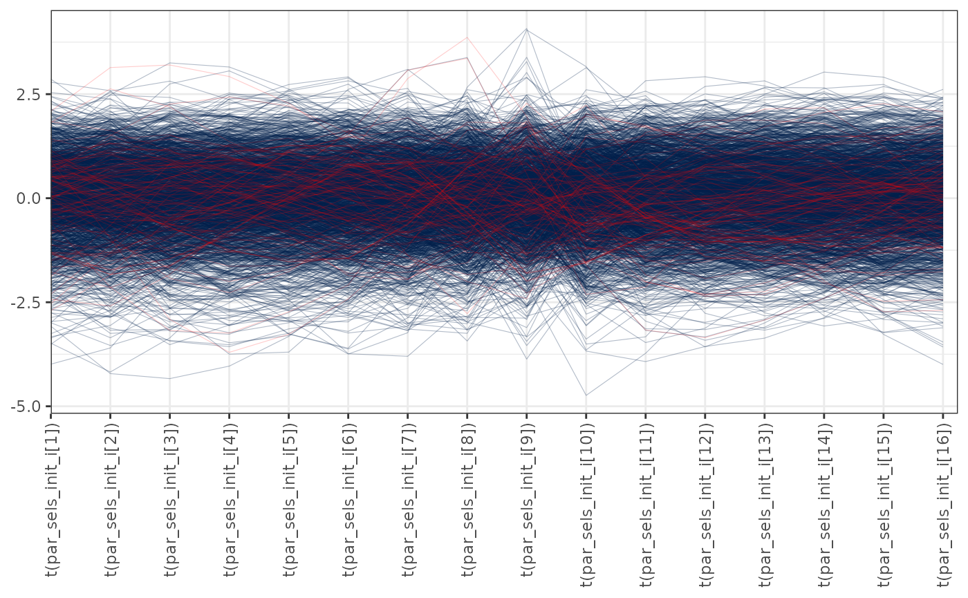
pars <- paste0("par_sels_change_i[", 130:140, "]")
mcmc_parcoord(x = mcmc1, pars = pars, np = nps,
              transform = function(x) {(x - mean(x)) / sd(x)}) +
  theme(axis.text.x = element_text(angle = 90, vjust = 0.5, hjust = 1))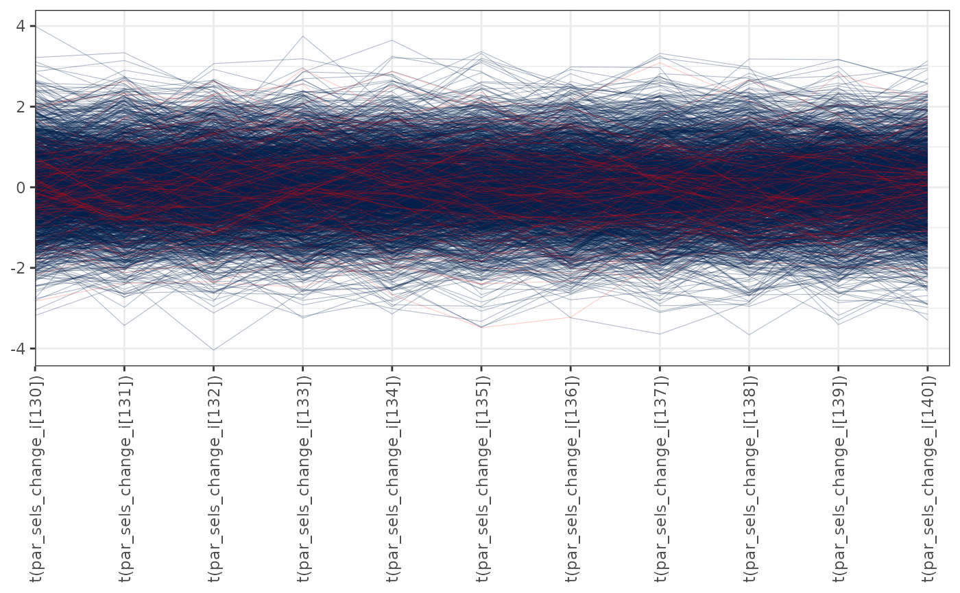
Obtaining samples from reported quantities
When samples from the posterior distribution are obtained using
tmbstan, only the model parameters can be accessed directly
from the stanfit object (i.e., derived quantities such as
par_B0 or M_a cannot be accessed directly).
Accessing derived quantities must be done using the
get_posterior function, for example:
par_B0 <- get_posterior(object = obj, posterior = mcmc1, pars = "par_B0")
# par_B0 <- get_posterior(object = obj, posterior = mcmc1, pars = "M_a",
#                         option = 2)
tail(par_B0)
#> # A tibble: 6 × 5
#>   chain  iter    id output    value
#>   <dbl> <dbl> <dbl> <chr>     <dbl>
#> 1     2   995     1 par_B0 7791000.
#> 2     2   996     1 par_B0 9253220.
#> 3     2   997     1 par_B0 8727151.
#> 4     2   998     1 par_B0 9661404.
#> 5     2   999     1 par_B0 9231579.
#> 6     2  1000     1 par_B0 8073366.
Leave-one-out information criterion
The leave-one-out information criterion (LOO IC) can be used for model diagnosis (e.g., identifying specific problematic data points), model selection, and model averaging:
if (FALSE) {
  loo1 <- get_loo(data = Data, object = obj, posterior = mcmc1)
  save(loo1, file = "loo1.rda")
} else {
  load("loo1.rda")
}

print(loo1)
#>
#> Computed from 2000 by 5388 log-likelihood matrix.
#>
#>          Estimate     SE
#> elpd_loo  -6082.2  769.9
#> p_loo       229.5   20.4
#> looic     12164.5 1539.8
#> ------
#> MCSE of elpd_loo is NA.
#> MCSE and ESS estimates assume MCMC draws (r_eff in [0.4, 1.3]).
#>
#> Pareto k diagnostic values:
#>                          Count Pct.    Min. ESS
#> (-Inf, 0.7]   (good)     5324  98.8%   55
#>    (0.7, 1]   (bad)        50   0.9%   <NA>
#>    (1, Inf)   (very bad)   14   0.3%   <NA>
#> See help('pareto-k-diagnostic') for details.
The POPs are excluded from the plot because there are so many of them.
plot_loo(x = loo1, exclude = "pop")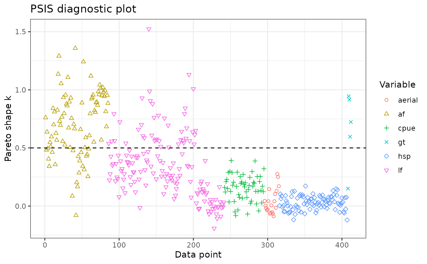
Posterior predictive plots
Compare the optimised results to the posterior distribution.
plot_cpue(data = Data, object = obj, posterior = mcmc1)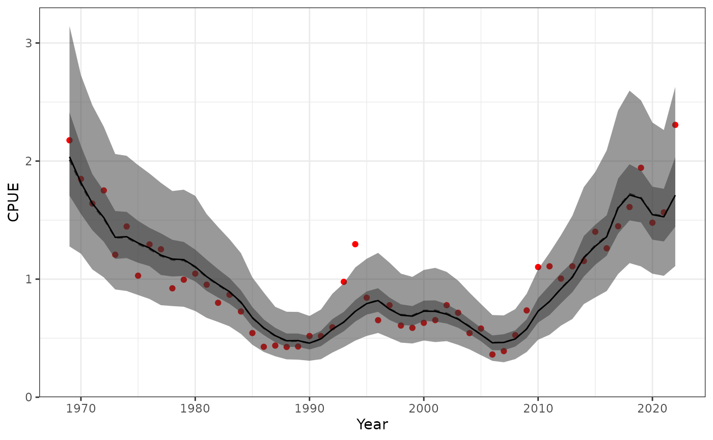
Fit to CPUE showing the 95% credible interval of the posterior and posterior predictive distribution.
plot_af(data = Data, object = obj, posterior = mcmc1, ncol = 4)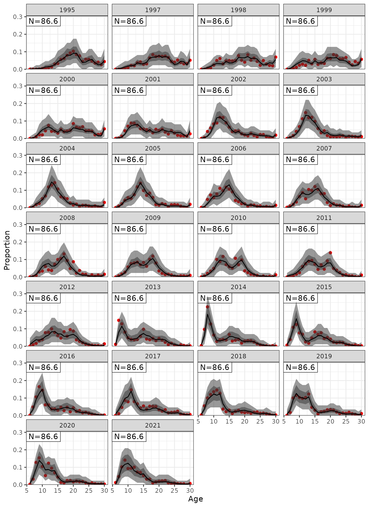
Fit to AF showing the 95% credible interval of the posterior and posterior predictive distribution.
Plots of reported quantities
plot_natural_mortality(data = Data, object = obj, posterior = mcmc1)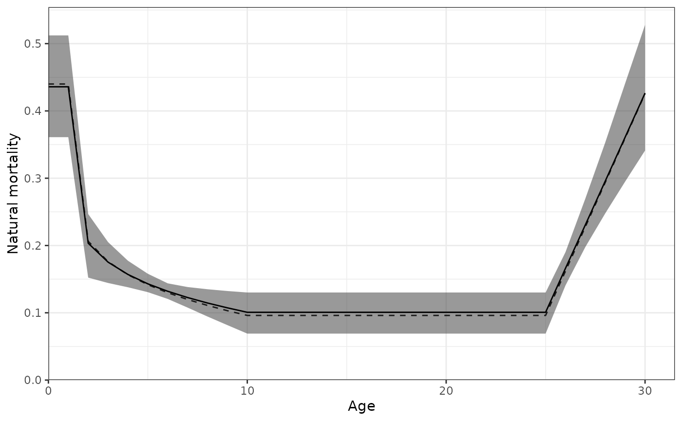
Natural mortality (M) by age showing the 95% credible interval.
plot_biomass_spawning(data = Data, object = obj, posterior = mcmc1,
                      relative = FALSE)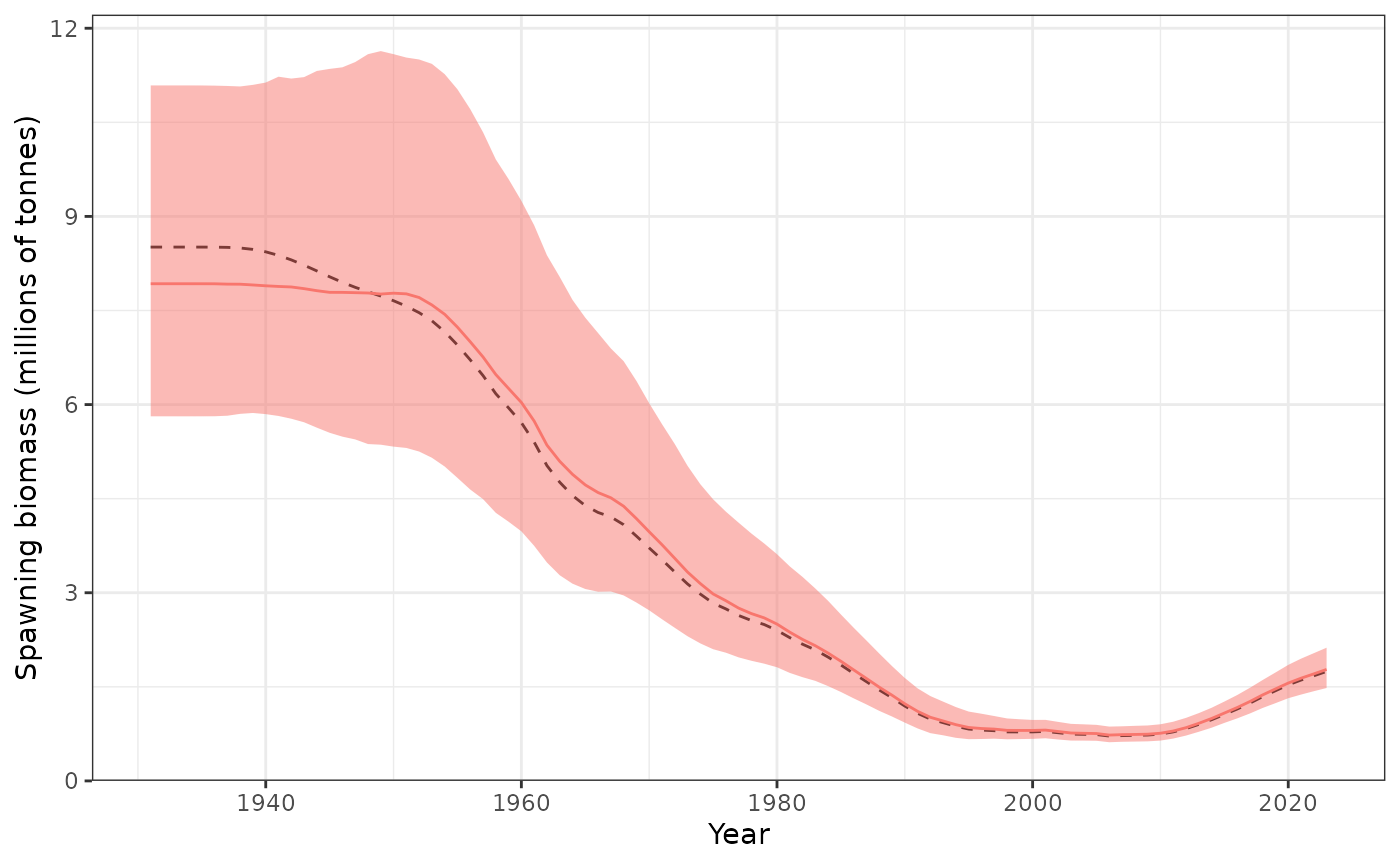
Spawning biomass (tonnes) showing the 95% credible interval.
plot_recruitment(data = Data, object = obj, posterior = mcmc1)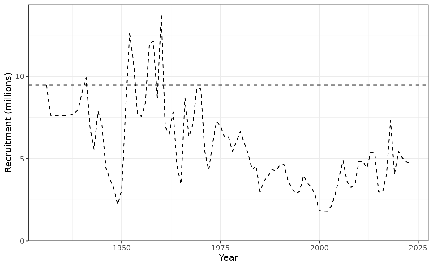
Spawning biomass (tonnes) showing the 95% credible interval.